Is My NGO Having a Positive Impact?

This post is jointly authored by David Evans and Bruce Wydick.

A daunting question faced by many non-government organizations (NGOs) involved in poverty work is—after all the fundraising, logistical work, direct work with the poor, and accounting is all done—one naturally wonders: Is my NGO having a positive impact? Indeed, as a recent Guardian article highlighted, “If the [NGO] sector wants to properly serve local populations, it needs to improve how it collects evidence.”  Donors are also increasingly demanding evidence of impact from NGOs, no longer just the large funders, but the small individual donors as well. 
 

This blog post is intended for development practitioners, specifically those of you without an overload of formal training in economics or statistics, but who want to carry out simple but valid impact studies on your work. There are whole books on this, of course, but here are a few simple principles to get you started.  
 
Most NGOs are good at measuring outcomes on their beneficiaries.  This is a step in the right direction. But to really measure impact, we need something in addition to beneficiary outcomes.  The key to carrying out a valid impact study is the generation of a counterfactual, or what would have happened to your beneficiaries if your program had not existed when they (hopefully) benefited from it.  Valid impact studies are essentially all about generating valid counterfactuals.
 
Let’s think about two common ways that NGOs try to estimate program impact.
 
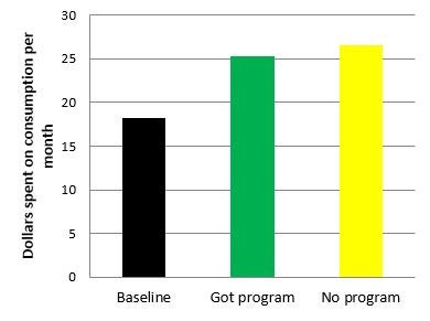
Before and After. One way is by taking baseline data on these program beneficiaries and then collecting more data on them after the intervention.  The counterfactual that is assumed in a before-and-after study is that without the program, the beneficiaries would have continued at the same level as at baseline. But the problem with this is that changes created by the program are often confused with changes that would have affected the program beneficiary over time anyway.  For example, the general economic climate might have improved since the baseline study. Then much of what you would attribute to impact is merely a rising tide lifting all boats. This was the case with a recent evaluation of providing cash transfers in Tanzania. The people receiving transfers significantly increased their food consumption (yay!). But it turned out that others, who weren’t receiving the transfers, had increased their food consumption just as much. In this case, the before-and-after study overstated the impact of the organization’s work. 

In Tanzania, comparing consumption for households receiving cash support before and after the program was misleading, since households without the program also increased their consumption.

Conversely, things in general may have gotten a lot worse, in which case you would understate it. In Nicaragua, a cash transfer program took place during an economic downturn: Consumption for participants rose while everyone else’s consumption was falling. Simply comparing the modest rise for participants since baseline would have greatly underestimated the full impact of the program.
 
Moreover, sometimes people choose to become involved with an NGO when they face certain opportunities, like when the timing of an economic opportunity drives someone to take a microfinance loan. Here the borrower would have been at least somewhat better off whether or not the non-profit was there to lend a helping hand. Indeed recent research finds that about three-quarters of apparent microfinance impact is an optical illusion from before-and-after observations. In summary, before-and-after studies don’t generate a valid counterfactual and therefore don’t generate valid measures of a program’s impact.
 
Beneficiaries and non-beneficiaries. Other NGOs sometimes measure impact by comparing program beneficiaries to non-beneficiaries.  The assumption here is that the condition of someone who is not affected by the program represents a counterfactual to a program beneficiary.  But data from non-beneficiaries don’t establish a valid counterfactual either.  Non-beneficiaries may lack the hidden qualities that induce a beneficiary to be part of the program.  These hidden qualities may be positively correlated with self-selection, in which case you would overestimate program impact.  They can also be  negatively correlated with self-selection such as when someone approaches an NGO for help in a time of crisis, in which case you would underestimate impact.  But either way you are likely to “mis-estimate” impact by trying to make these comparisons.  Estimating your program’s impact by comparing beneficiaries to non-beneficiaries is likely to produce very misleading results.
 
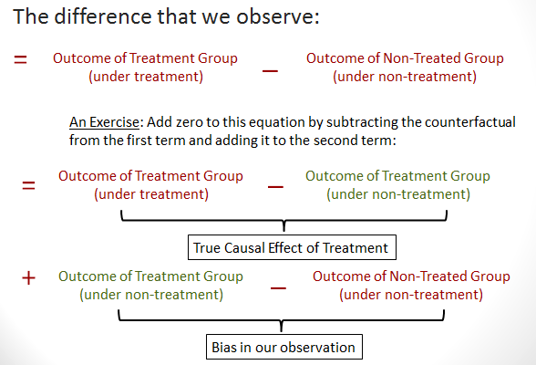
Indeed everything that we observe—before-and-after differences or differences between beneficiaries and non-beneficiaries consists of the true impact and the bias in our observation.  We can see this easily by both subtracting and adding the counterfactual to this difference as seen in the diagram below.
Getting it right. So how do you generate valid counterfactuals?  This is the trick that lies behind all good impact studies.
 
The general principle behind generating valid counterfactuals to the work of your NGO is to try to replicate the qualities of your beneficiaries (both observed and unobserved) to create a group of people that statistically replicates your beneficiary group but didn’t receive your intervention.  A few good ways to do this are through (A) Embedding a randomized experiment within the relatively normal scope of your work; (B) Using an arbitrary eligibility cutoff that you employ to select beneficiaries to create counterfactuals around that cutoff; (C) Using a combination of before-and-after & beneficiaries vs. non-beneficiaries, called a “difference-in-differences.”  Here we provide some examples of each.
 
(A) Embed a Randomized Experiment into your Work.  Let’s suppose your organization provides school fees for children of low-income families in Tanzania.  You have X amount of resources from donations, and with X, much as you would like to, there is no way you can help every child in Tanzania.  Hard choices have to be made.  One way to do this is through a kind of “assessment + triage + lottery.” 
 
First, assess the basic conditions of each of the children in your area of operation who you might consider for your program, simple measures of household poverty, health status, “at-risk” status, and so forth.  Based on these measures, order the children along a continuum of how likely their decision to attend school would seem to depend on receiving the school-fee subsidy.  Then divide the children into three groups:  1) Those whose schooling decision would almost certainly respond to the school-fee subsidy; 2) Those who might be influenced to attend school from the subsidy; 3) Those unlikely to benefit from the subsidy (either because they would attend school even if they didn’t get the subsidy, or because they wouldn’t attend school even if they did get the subsidy).  By the way, this approach will not only help you to measure impact, it is also likely to help you increase it.
 
Let’s suppose you have enough resources for category 1 children, plus some left over for other children, but not enough for every child in category 2. So after eliminating the children from category 3 from consideration, you provide the subsidy to every child in category 1.  Then you announce that to give every child in category 2 “a fair and equal chance” at a school-fee subsidy, you will hold a public lottery to allocate these spaces.  Let’s assume that 40% of category 2 children are chosen through the lottery.  To measure your impact, you would then measure outcomes (perhaps at different points in time) between the 40% of the category 2 children that were chosen, and an equal number of randomly chosen category 2 children who were not selected by the lottery.  Across your chosen impact measures (school attendance, reduction in child labor, learning, etc.) the difference between these is your measure of average impact.  Dividing this difference by the standard error of your estimate, gives you a t-statistic, which if greater than 1.96, indicates statistical significance at the 5% level of confidence, which is statistics-speak for indicating a reasonably high level of certainty that the result is not just a result of random chance.
 
Another kind of experiment.  Even if everyone is allowed to participate, another type of experiment that can be run with this type of program would be one in which certain households chosen from a larger sample of eligible households randomly receive an invitation for their children to participate.  Suppose your response rate among invited households is m and among the uninvited households it is n.  (If you did a good promotion, then m should be a lot bigger than n, which it needs to be for this to work.) Then, after a period of time, you survey over your impact measures over all members of both groups, the randomly invited and non-invited.  If we call the average outcome among all of the invited group M and the average impact among all of the not-invited group N, then an estimate of the impact of the program is (M – N)/(m – n).  Once again, you divide this estimate by a standard error to be confident that the difference you observe isn’t just by chance.
 
(B) Use an Eligibility Cutoff.  Let’s suppose you don’t feel like running an experiment, but you assign benefits from your program based on some indicator. For example, you manage

• an agricultural project that provides seeds to any farmer with less than 0.5 square kilometers of land, but not to any farmer who has more land than that; or
• an education project that provides school uniforms to all students with at least an 80% on last year’s end-of-year exam; or
• a poverty-alleviation project that gathers indicators on 10 assets from households in each village and provides a package of support to households that have 5 or fewer of those assets.

 
In this case, you can use what is called a “regression discontinuity design.” Consider the first example, where you provide seeds to farmers with less than 0.5 square kilometers of land. Of course, if we compare farmers with almost no land, say 0.1 km², to farmers with lots of land (say, 50 km²), then we’d run into the same problem as above with beneficiaries and non-beneficiaries. They are so different even before the program that no difference in agricultural yields after the program can really be attributed to the program.
 
But think about the farmer with 0.4 km² (who does receive the seeds) and the farmer with 0.6 km² (who doesn’t). Those farmers are pretty similar before your seed program. They’re both small farmers: One just happens to fall below your cut-off and the other just happens to fall above it. Even just evaluating your program by comparing those farmers who are above the cut-off (but close to it!) and not benefiting from your program with the farmers below the cut-off (but close to it!) will give you a much better estimate of the impact than simply comparing beneficiaries and non-beneficiaries in general.
 
That said, those two farmers still aren’t identical, even before you distribute the seeds. The farmer with 0.6 km² may be a little more entrepreneurial than the farmer with 0.4 km² (after all, maybe that’s why she has 0.2 more km²).  So the best way to do this would be to run a simple regression analysis that allows you control for the amount of land each farmer has (and perhaps other variables) while making the comparison on either side of your eligibility rule.
 
For this method to work, you really need a good number of beneficiaries near the cut-off. Keep in mind as well that this method tells you how effective your program is for people who are near that cut-off. So it doesn’t necessarily tell you how well the program works for farmers with micro-plots of 0.1 km². But the farmers near the cut-off can be very important: If you are thinking of expanding the program to farmers who have less than 0.6 km², then understanding how well the program works near there is the best information you can have.
 
(C) Combine before/after and beneficiaries/non-beneficiaries.  Although studies based on “before-and-after” and “beneficiaries vs. non-beneficiaries” each contain substantial weaknesses on their own, when combined they can produce substantially more reliable results.  Suppose you manage a program that provides chickens (to eat, to breed, and to sell) to the poorest households in a community. You want to know whether beneficiary households have higher incomes after receiving these chickens. You can’t just compare them before and after receiving the chickens. If you do, you’re assuming their income would have stayed just the same without the chickens, when people’s incomes can fluctuate for many reasons. You can’t just compare them to other community members who don’t get the chickens, since those who receive chickens may still be among the poorest, even if the chickens improve their incomes.
 
The “difference-in-differences” method improves on the before/after and the beneficiary/non-beneficiary comparison by using both at once. You look at the beneficiaries before and after; let’s say their incomes rise from 100 pesos to 200 pesos monthly. You also look at the non-beneficiaries before and after. Imagine their incomes also rise, just because the community had good rains, from 300 to 350 pesos. So, we see the change in income for the beneficiaries (100 pesos, from 100 to 200). But we also see the change in income for the non-beneficiaries (50 pesos, from 300 to 350). We assume, in this case, that the change for the non-beneficiaries is what would have changed for the beneficiaries without the program.
 
The effect of the program would be 100 (the actual change for beneficiaries) minus 50 (what we think would have happened to beneficiaries without the program, as judged by non-beneficiaries), or an improvement – due to the program – of 50 pesos monthly. The method is called “difference in differences” because we measuring the difference between two differences (the change over time among beneficiaries versus the change among non-beneficiaries).
 
This method gives an accurate measure of impact only if you have good reason to believe that the income of the beneficiaries and non-beneficiaries would be growing at the same rate in the absence of the program. The best way to check if this is likely is to look at how quickly consumption grows for both groups before the program is introduced.
 
Take away
This is just a taste of these methods, but the objective here is to show you that it is indeed possible to evaluate your programs, and you don’t need to have a PhD for simple evaluation methods. If you want to learn more, here are some resources for you.

• The World Bank has a free non-technical book on impact evaluation by Paul Gertler et al., available here. It’s also available in French, Portuguese, and Spanish.
• The World Bank has also published a useful book that assumes a basic knowledge of regression analysis, The Handbook on Impact Evaluation, by Sahidur Hkandker, Gayatri Koolwal, and Hussain Samad that is available free by pdf.
• Glennerster and Takavarasha have a great book called Running Randomized Evaluations, which is a great resource for doing randomized experiments.
• The Inter-American Development Bank’s Impact Evaluation Hub has more on methods, as well as checklists and templates for every stage of an impact evaluation.