However, in hindsight, it does seem like it would have been a good idea for the authors of the study to conduct multiple inference adjustments and report them in a short and simple paragraph – especially if they knew they’d be giving media interviews about their findings. Sadly, in today’s environment, one of the jobs of the academic researcher is to prevent the journalist from overselling or misreporting her results as much as possible. And, when it still inevitably happens, then at least you can point to that sentence in your paper…
What would have happened had they done so? Not only could they have emphasized the change in obesity in a different age group, but they could have also told us under what conditions we might assign some credibility to the idea that obesity among 2-5 year-old children dropped between 2003-2004 and 2011-2012. Let’s see how:
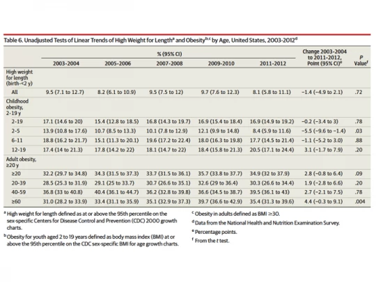
In the study, which is a descriptive analysis of repeated cross-sectional data, there is only one table that we’re interested in, which reports changes over time (see Table 6 from the study below). In this table, obesity is reported for six age groups (2-5, 6-11, 12-19, 20-39, 40-59, and over 60) for five time periods (03-04, 05-06, 07-08, 09-10, and 11-12), with unadjusted p-values from t-tests reported only for the longest-term comparison (i.e. the change between 03-04 and 11-12). That is six t-tests.* Since you run a risk of making a Type 1 error each time you conduct a t-test, the unadjusted p-values overstate confidence in the estimates. Oster suggests that the authors could have used a Bonferroni adjustment – the most rudimentary adjustment in general use – which would have required the authors to consider a 0.008 threshold rather than 0.05. Since the 5.5 percentage point (pp) drop in obesity among children aged 2-5 has a p-value of 0.03, it would not have cleared this hurdle. However, the 4.4 pp increase among those aged 60 and older would have easily – with its p-value of 0.004 (a bit more on this below).
The advantage of using a Bonferroni correction is in its simplicity (we teach it in introductory statistics), but results in poor power: in other words, you put all your worry into avoiding any Type I error at the cost of Type 2 errors. My ‘go to’ source on the topic of multiple inference corrections, a paper published in JASA by Michael Anderson in 2008, suggests that while it is necessary to do this when the stakes are high (i.e. the cost of making a Type I error is huge because the government or the Gates Foundation may put billions of dollars into a prevention approach based on your findings), it is likely to be overly restrictive in a more exploratory setting. In such cases, Anderson argues that you might tolerate some Type I errors for greater power in your study. I’d say that this probably applies to the JAMA article, which is a descriptive analysis of obesity trends in the U.S. and is not evaluating any one intervention or program.
So, what are those alternative techniques? Bonferroni adjustments belong to the family of approaches that control the family-wise error rate (FWER). Anderson (2008) describes a step-by-step algorithm to conduct the free step-down resampling method (Westfall and Young 1993), which increases power and, unlike Bonferroni, allows for dependence between outcomes (the paper is very accessible and easy to understand – after all I did – so don’t be scared to read and utilize). This method ensures that the probability of falsely rejecting at least one hypothesis is less than alpha (say, 0.05 or 0.10), but both approaches under FWER still aim to limit the probability of making any Type I error.
In contrast, the approach to control the false discovery rate (FDR), the expected proportion of rejections that are false (i.e. Type I errors), “…formalizes the trade-off between correct and false rejections and reduces the penalty to testing additional hypotheses.” (Anderson 2008, ppg. 1487) A simple method for controlling the FDR is a procedure proposed by Benjamini and Hochberg (1995), described nicely both in Anderson (2008) and also in this paper by Fink, McConnell, and Vollmer published in the current issue of the Journal of Development Effectiveness. It essentially involves ordering the p-values in ascending order: in the case of the JAMA study, the p-values in Table 6 are such that p1=0.004; p2=0.03; p3=0.20; p4=0.20; p5=0.78; p6=0.88, where we index i=1 through 6; m=6, the total number of tests; and q=0.05, our desired FDR. Then, starting from the highest p-value, you check whether pi
Anderson (2008) also describes (and proceeds to utilize in his reanalysis of the effects of early childhood programs in the U.S.) another procedure, proposed by Benjamini, Krieger, and Yekutieli (2006) that further sharpens this procedure and makes it even less conservative. The intuition is as follows: because you’re trying to keep the proportion of false rejections below a certain rate in expectation, the more “incorrect” null hypotheses you have the more power you get. You don’t know the number of incorrect hypotheses, but you can predict them to be the hypotheses tests with very small p-values. So, the fact that you have a p-value equal to 0.004 among your six p-values (almost certainly a correct rejection of the null hypothesis) may give you enough leeway to also reject a hypothesis test with a p-value=0.03 (turns out here that it doesn’t). This procedure, BKY (2006), is as easy as BH (1995) described above, but it has two stages instead of one. You can conduct both BH and BKY in your head (or the back of an envelope) while looking at a table like Table 6 in the JAMA study – if, that is, the authors weren’t kind enough to have already done it for you.**
So far, we have the following. With a threshold of 0.05, unadjusted p-values in Table 6 of the JAMA study would have rejected two of the six null hypotheses on obesity trends in different age groups. The NYT piece focused on one of these (the reduction among children) and ran with it (I don’t know why they ignored the increase among the elderly — even with one of the study authors mentioning it in her quote). With a FWER-type correction, like Bonferroni, or a one-stage or two-stage FDR correction, that number goes down to one: you’d still be happy to report a good possibility of an increase in obesity rates among those 60 and older, but not put much weight in a decrease among children, aged 2-5. Emily Oster focused on the latter in her piece but does not mention the former, either.
What if you wanted to control FDR at 0.10 rather than 0.05? In other words, what if you were happy with 10% of your rejections, on expectation, being false. After all, 0.10 is not an uncommon threshold for statistical significance in economics. Turns out that you’d now reject both H1 and H2. This is because 0.004Stata code to calculate these on his website). My back of the envelope calculation is that the q-value is approximately 0.025 for the hypothesis test on the elderly and 0.09 for that among children.
Reading the findings of the JAMA article in this way, I personally would be at least a little bit intrigued to think about the underlying reasons why such changes (in opposite directions) in obesity might have occurred in the U.S.. Emily Oster conducts some of the further analysis in her piece on fivethirthyeight.com. There is little doubt that the start and end dates are arbitrary and one would like to see changes show up for other periods: if starting a little earlier and ending a little earlier wipes out the findings, we’ll start becoming more dismissive. The authors of the study could have saved everyone a lot of time and reported multiple inference corrections in a paragraph not much longer than the one in which they declare not having undertaken these corrections. Maybe next time… The hope is that some of you will do so in your own papers!
* The authors also report p-values for childhood (ages 2-19) and adulthood (ages 20 and above), as well as a measure of high weight for height for children under 2. The higher grouping of ages is really not necessary for the argument and the authors could have omitted these from this table or their analysis. High weight for height seems like a different outcome than obesity, and will ignore it here as well. Oster, who suggests a correction for six tests, seems to be implicitly making the same judgment. Furthermore, there actually are 60 tests of change over time that could be conducted (10 for each age group) in Table 6, and a different analysis might report adjusted values for all those 60 comparisons. Since the authors do not report any p-values for shorter-term comparisons since 2003-04 and because shorter term comparisons are presumably of lower interest, I ignore this here and focus on making corrections for the fact that six hypothesis tests were conducted for age subgroups. Finally, Oster makes the point that the sample sizes get small for subgroup analysis. In such cases, it is a good idea to report nonparametric permutation tests rather than standard t-tests that rely on asymptotic theory. The authors of the JAMA study have not done this, perhaps because none of the sample sizes for the six age groups is below 100.
** The BKY (2006) paper goes on to describe a similar multiple-stage procedure. It is important to note that FDR procedures are valid for independent or positively-dependent p-values and researchers dealing with negatively-dependent p-values may refer to Benjamini and Yekutieli (2001) for conservative modifications of the BH (1995) procedure.

Join the Conversation