What Are We Estimating When We Estimate Difference-in-Differences?

Difference-in-differences estimation is one of the most widely used quasi-experimental tools for measuring the impacts of development policies.  In 2018, I calculate that more than 5 percent of articles published in the Journal of Development Economics used a difference-in-differences (or “DD”) methodology.  In DD estimation, a researcher compares the change in outcomes in a (non-random) treatment group before vs. after treatment to the change in outcomes in a comparison group over the same time period (even though the comparison group never received treatment).  The figure below illustrates the basic idea.

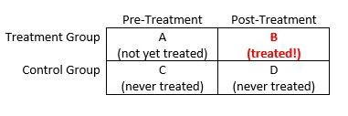
The DD estimate of the treatment effect is: (B – A) – (D – C).  Intuitively, pre-treatment differences between the treatment group and the comparison group reflect selection bias, while pre-period vs. post-period changes in outcomes within the comparison group reflect time trends.  The DD approach removes these confounds (under certain assumptions) by differencing them out, leaving us with a credible quasi-experimental estimate of the treatment effect of interest.  A more detailed overview of DD methods is available here.

The DD approach is often used to estimate the impacts of policies that are implemented at different times in different regions, for example policies like Medicaid and food stamps that were implemented in different times in different U.S. states.  In development, this approach was recently used by Jesse Antilla-Hughes, Lia Fernald, Paul Gertler, Patrick Krause, and Bruce Wydick to study the impacts of infant formula on child mortality in low- and middle-income countries.  In such settings, researchers typically implement the DD using two-way fixed effects models controlling for both period-specific and unit-specific shocks.

Though the two-way fixed effects approach to DD is widely used, the formal justification for treating it as a DD estimator is often fairly ad hoc.  A recent working paper by Andrew Goodman-Bacon, an Assistant Professor of Economics at Vanderbilt University, looks under the hood of the two-way fixed effects approach to DD estimation.  Goodman-Bacon shows that any two-way fixed effects estimate of DD relying on variation in treatment timing can be decomposed into a weighted average of all possible two-by-two difference-in-differences estimators that can be constructed from the panel data set. 

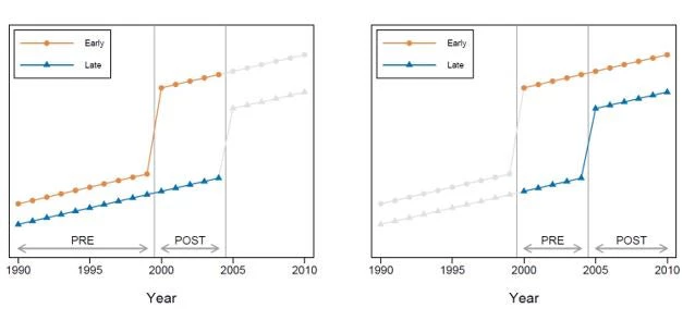
Consider a (hypothetical) data set comprising two types of countries:  one group that made primary education free in 2000, and another group that made primary education free in 2005.  Call the first group the “early” countries and the second group the “late” countries. Suppose you had data on primary school completion rates every year from 1990 to 2010.  Such a data set allows for two distinct DD comparisons.  First, we could focus on the period from 1990 to 2004 (the left panel in the figure below).  In that time frame, the late adopter countries are “never treated” in the sense that they do not implement free primary education – so they can be used as a comparison group to estimate the impact of free primary on test scores in the early adopter countries.  However, we can also construct a second DD estimate of the treatment effect of free primary school by focusing on the years 2001 to 2010.  During that period, the treatment status of the early adopters never changes – they remain treated throughout – so they can be used as a comparison group to estimate the impact of free primary on test scores in the late adopting countries. 

Goodman-Bacon shows that any two-way fixed effects estimate of DD with variation in treatment timing can be decomposed in this way.  It is a weighted average of (1) comparisons between (relatively) early adopters and later adopters over the periods when the later adopters are not yet treated, (2) comparisons between early adopters and later adopters over the periods when the early adopters are treated – so that they can be used as a comparison group for the later adopters, and (3) comparisons between different timing groups (e.g., early adopters or later adopters) and the never-treated group, if there is one. 

Though interesting in its own right, this decomposition has several important implications.  First, two-way fixed effects estimates of DD that rely on variation in treatment timing only recover the average treatment effect when treatment effects are homogeneous.  When treatment effects are heterogeneous across units, OLS over-weights units with more variance in treatment status in order to achieve a more precise estimate of the treatment effect.  Hence, units that are treated near the middle of the evaluation window receive relatively more weight.  If one wishes to estimate the average treatment effect on the treated, some sort of re-weighting is required.

Second, and more troublingly, DD estimates are biased when treatment effects change over time within unit.  Intuitively, this occurs because already treated units serve as controls in some of the two-by-two DDs underlying the weighted average.  When treatment effects are not constant over time (so, for example, the treatment effect in the first year after treatment differs from the treatment effect five years after treatment), using already treated units as controls necessarily biases estimates of the treatment effect (by introducing a term representing the change in the treatment effect on the already treated units).  In such situations, Goodman-Bacon’s analysis shows that two-way fixed effects estimators are not appropriate, and alternative approaches (e.g., event study estimation) should be used. 

In light of this, it is important to check whether common trends are satisfied in any panel data set being used for DD analysis.  When treatment turns on at different times, one way to do this graphically is to re-center and stack all the possible two-by-two DD comparisons.  Critically, identification relies on common trends both before and after treatment – as discussed above.  The good news is that, because of the re-weighting of the underlying two-by-two DD estimators, some violations of common trends are worse than others.  Goodman-Bacon provides instructions for testing “variance-weighted common trends” to assess the severity of any observed deviations.

If this all sounds like it raises the bar for DD analysis: it does.  Fortunately, there’s already a Stata command to help you implement the Goodman-Bacon’s DD decomposition.  Search for “bacondecomp” and you will find Goodman-Bacon, Goldring, and Nichols’ (2019) helpful tool for decomposing and plotting the underlying variation in your two-by-two DD estimates.