Motivation
A lot of us have been getting the suggestion: “Attrition seems like it might be an issue here — can you restrict your analysis to a balanced panel?” What assumptions are needed for this to be unbiased while estimates not restricting to a balanced panel are biased? Unclear! Will Lee bounds fix my attrition problem? Who’s this MIPO anyway? This is a legitimate source of confusion—so it was time for a Development Impact blog post (and a new Shiny dashboard!) about this.
Attrition
Attrition is a common scourge of randomized control trials, threatening our “gold standard” (sic) estimates with pesky bias. While we know that random assignment to treatment ensures that there is no difference on average (besides the treatment) between treatment and control individuals, attrition has the power to change this for the set of individuals that we actually observe. In particular, this can occur when the individuals that attrit from the treatment group are different from the individuals that attrit from the control group, leaving us with a set of observed individuals that are no longer identical in treatment and control.
There has of course been quite a bit of literature on this in this very blog. Berk summarized a number of approaches to attrition. When attrition is independent of potential outcomes (MIPO), then attrition does not generate bias. Alternatively, when attrition is independent of potential outcomes conditional on certain baseline covariates (MIPO | X), then standard conditional-on-observables approaches (e.g., PSM) can be used to correct for bias. Additional restrictions on attrition leave estimates biased, but can yield informative bounds on treatment effects, and these bounds can be sharpened using similar conditional-on-observables approaches. David pointed out that these bounding approaches can be combined with increasing the number of attempts needed to track respondents for additional precision. However rare differential attrition turns out to be, it appears more frequently when the treatment is sufficiently large that it might cause individuals to become more (or less) likely to attrit.
While all this provides a bouquet of approaches to tackle attrition, it left us wondering what patterns of attrition cause us to need one or another. In particular, whether “balancing our panel” could ever really correct for this…
Dashboards as the econometric sandbox
To answer these questions, we set out to create a simple to use tool for us to experiment with different methods under different assumptions about the data generating process. We started by simulating data, to see which specifications work when and under what assumptions they break down (e.g., what patterns of attrition bias which estimates?).
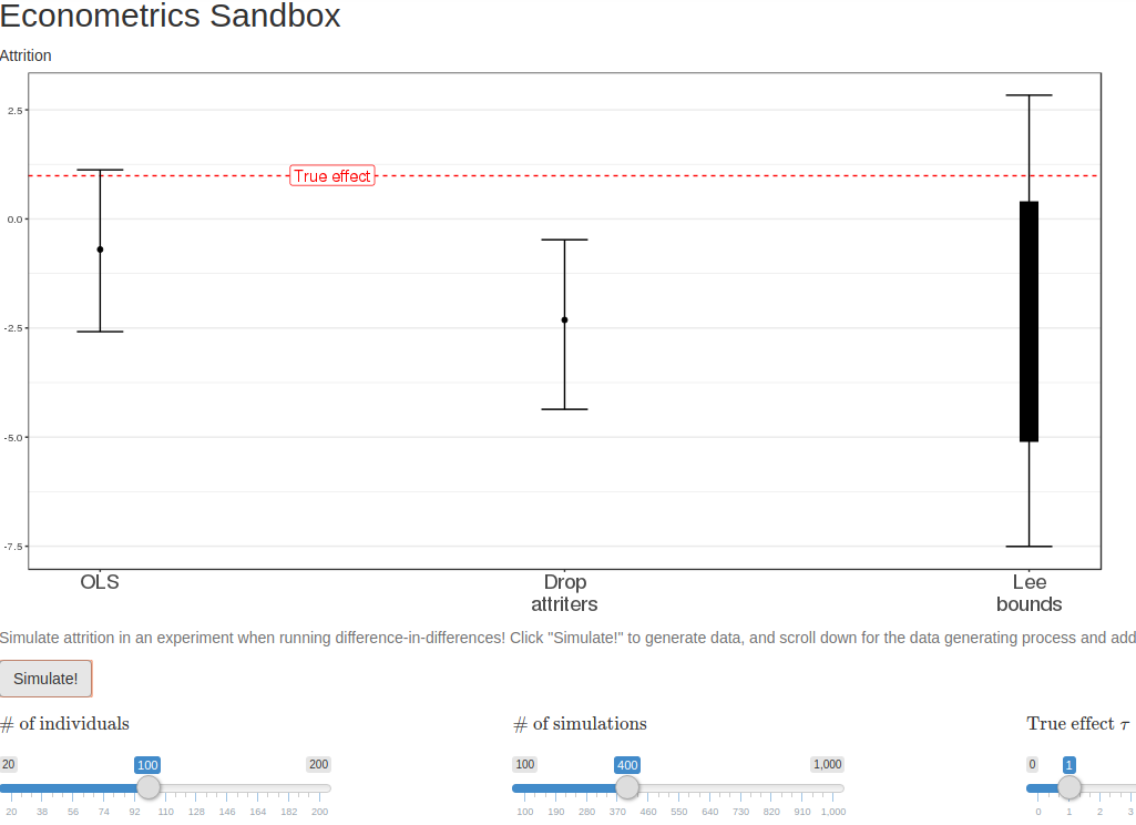
To share these simulations without requiring a bunch of supplementary steps to download and execute code… we created a dashboard! The dashboard does three things. First, it enables varying the parameters of the data generation process. Second, it runs three simple approaches to dealing with attrition in a simple two period difference-in-differences setup: ignoring it, dropping attriters, and implementing Lee bounds on the first differences. And third, it visualizes and compares the estimates coming out of each of these models. We found this useful as an exploration tool to understand what assumptions underlie different approaches to handling attrition in an experiment.
Data generating process
A series of sliders shift key components of the data generating process. These include the number of individuals, the true effect of the intervention, properties of the structural errors, and, crucially, patterns of selection into attrition and attrition probabilities. The latter two determine the characteristics of the individuals who attrit, which crucially affects bias — do attriters have different outcome levels? do they have differential growth? do individuals who attrit when assigned to control differ from individuals who attrit when assigned to treatment?

To highlight the simple mechanics of attrition, we restrict to the canonical two period difference-in-differences case with random assignment to the intervention, where attrition occurs only in the post period. In doing so, we also ignore the possibility of controlling for observables (which we discussed briefly above). Additionally, this ignores considerations that may be more common with panel data with additional periods (when dropping attriters and including individual fixed effects are not identical) or non-experimental approaches.
Models
Next, we run three models on the simulated data. The first is a difference-in-differences (“OLS”). Letting \( y_{it} \) be the outcome of interest observed for unit \( i \) in period \( t \) (where \( t \) is 0 for the pre-period and 1 for the post-period), \( \text{Treated}{i} \) indicate that unit \( i \) was treated in period 1, and \( \text{Post}_{t} \) be an indicator for period 1, we estimate
\[ y_{it} = \alpha + \beta \text{Treated}_{i} \times \text{Post}_{t} + \gamma_{1} \text{Treated}_{i} + \gamma_{2} \text{Post}_{t} + \epsilon_{it} \]
Here, \( \beta \) is our difference-in-differences estimator: the difference in average outcomes for treated units in the post-period relative to the pre-period, minus the difference in average outcomes for control units in the post-period relative to the pre-period. However, when some units are not observed in the post-period, these averages are not over a consistent set of units; as discussed above, this may be particularly problematic when treatment itself causes some units to attrit (or not to attrit).
Second, we instead restrict to units that do not attrit. This is the most familiar difference-in-differences case, and here the above difference-in-differences estimator, two way fixed effects, and first differences are all equivalent. We therefore estimate (dropping attriters)
\[ y_{i1} - y_{i0} = \alpha + \beta \text{Treated}_{i} + \epsilon_{it} \]
While this drops units that attrit, when attriters are different in the treatment and control group, selection bias may still bias this estimate.
Third, we apply Lee Bounds, a common approach to dealing with selection bias, which produces treatment effect bounds that are robust to differential attrition. These have been discussed in additional detail previously on the blog here and attrited by Berk here; in brief, these require a “monotonicity” assumption that there are no “defyer attriters” (e.g., if there is more attrition in the control group, there must be no individuals who were caused to attrit by treatment, similar to a “no defyers” assumption in instrumental variables).
Visualization, one click away!
Lastly, we plot the estimates from each of these models in the dashboard. All one needs to do is to click “Simulate!” to create a new simulation of data, run the three models, and plot the estimated coefficients (or bounds) and 90% confidence intervals from each model. Voilà!

Now let’s play… threats to identification!
Going back to our original motivation, what patterns of attrition cause bias in each of the three different approaches to estimation? To estimate the role of each, we used the dashboard to simulate data under differential attrition, and compare the effects we estimate to the true effect of the intervention. This way, if the effect we estimate is different from the true effect, we know this difference was actually caused by bias due to attrition.
We simulated four cases, visualized in the figure above. In each case, we set \( P(0) = 0.1 \) and \( P(1) = 0.4 \), so attrition is more likely in treatment than in control.
Differential attrition at random: First, when attrition is random within both control and treatment, all methods recover the true effect. Despite differential attrition, this is because the average observed outcome in each group in each period is unbiased for the true average outcome in that group. It’s hard for us to imagine empirically why this would be the case. However, one test of this could be looking at which baseline characteristics predict attrition or differential attrition; if none do, this may suggest that attrition is as good as random.
Differential attrition on levels (\( \beta_{2} = 1 \), \( \beta_{4} = 1 \)): Second, when attriters in the treatment group have relatively high outcomes, this biases OLS downwards, as OLS includes these attriting individuals in the pre-period treatment average but not in its post-period treatment average. However, the two approaches using within unit differencing do not have this bias. Note that this assumption is similar to a difference-in-differences assumption, that attriters have “parallel trends” with non-attriters within treatment and control. When attrition is on a single question (instead of for the entire survey), tests of “parallel trends” using other variables may be possible. However, similar to differential attrition at random, it is hard to imagine empirically why this assumption might hold.
Differential attrition on growth (\( \beta_{4} = 1 \)): Third, when attriters in the treatment group have relatively high growth in their outcomes, this biases all point estimates downwards. However, Lee bounds successfully cover the true treatment effect in this case. While this allows attriters to have fundamentally different levels and growth from non-attriters, it maintains a “monotonicity” assumption that every individual who would attrit under control will also attrit under treatment (or vice versa). This will be true if treatment strictly increases (or decreases) the probability of attrition for all individuals. This might be the case if treatment primarily (and monotonically) affects a single behavior that increases (or decreases) everyone’s likelihood of attrition, such as migration.
Non-monotonic differential attrition on growth (\( \beta_{4} = 1 \), \( \rho = -1 \)): Fourth, when attrition is non-monotonic and attriters in the treatment group have relatively high growth in their outcomes, then even Lee bounds fail to successfully cover the true treatment effect. In this case, the set of individuals who attrit under control is not a subset of the set of individuals who attrit under treatment. This could be the case if, for example, treatment causes some individuals to migrate but causes other individuals to not migrate, and these individuals differ in their potential outcomes. Were this true, one might also expect to observe nonmonotonic effects of treatment on attrition with respect to propensity to attrit in the control group (i.e., one could apply an endogenous stratification approach recently discussed on this blog to test for this).
Main takeaways
Which patterns of selection are plausible determines which methods can or cannot mitigate attrition issues. In many cases, these patterns of selection have testable implications, and it is often possible to tightly bound treatment effects even in the presence of endogenous attrition. Further, we were surprised that restricting to a balanced panel (our original motivation) could correct for bias under any set of assumptions, although we were wholly delighted to find that, as shown in the initial figure in this post, it is also possible that restricting to a balanced panel worsens bias!
Note: All codes from our Econometric Sandboxes blogposts are hosted here!


Join the Conversation