The use of historical data for economic analysis has been on the rise in recent decades. Persistence studies in particular have been essential in developing our understanding of how historical factors can contribute to present-day economic and social outcomes. In this literature, maps are often a key source of historical data. For example, many papers in the persistence literature rely on a historical regression discontinuity design (RDD) for their specification and hence require the extraction of historical boundaries from old maps. The seminal paper by Melisa Dell (2010) uses the historical Mita boundary to examine the long-run effects of an extensive forced mining labor system in Peru and Bolivia. Similarly, Cogneau et al. (2014) use the border between the French and British territories in colonial Togo and Ghana to analyze persistence in literacy and religious affiliations. A key challenge in this literature is to extract information from historical maps in a way that is accurate and easily reproduceable. However, in the absence of automated tools, researchers must often manually draw and digitize these borders, which may generate concerns about precision and accuracy.
In this post I discuss a method developed by Anna Peichel in her 2020 paper ‘Semi-Automatic Vector Extraction of Administrative Borders from Historical Raster Maps’, where she details a methodology to extract historical borders from maps. I provide an overview of her steps and how they can be used for digitization. I show how her methodology was employed on a 1925 map of Ouagadougou in the colonial Upper Volta-French Sudan by Dupas et al. (2023) and show its step-by-step evolution in the process. The final process in Dupas et al. (2023), described in Appendix D of the paper, further builds on this methodology by using ArcGIS, QGIS, Python, and Adobe Photoshop to automatize the process as much as possible.
Although one must keep in mind that in certain situations alternate methods may be more suitable, but for someone without extensive knowledge of GIS softwares, these steps provide a simple option that makes use of free software and could therefore be widely applicable.
Processing the Map
Historical maps often suffer from image quality concerns. The colors may be faded, and the objects often pixilated. In these cases, simple image processing can enhance the accuracy of the extraction procedure. Among the various possibilities, I find adjusting the image brightness and the contrast to be most rewarding. Brightness helps increase the visibility of the map elements, especially the darker ones. Contrast, on the other hand, allows you to increase the difference between the lighter and the darker areas of an image. This helps to differentiate the objects on the map from their background. Since the following steps focus on being able to extract a particular color from the map, any processing tool (GIMP, Adobe Photoshop) that would help enhance a particular color could potentially be helpful.
Extracting Color
The next step is to isolate only those elements from the map that you need to digitize. I use the free ‘Pixlr X’ website, where you can go to the cutout tools and use the ‘magic cutout’ feature. This allows you to click on the color that you want to isolate, and it then selects all the pixels of that color in your map. In other image processing softwares (such as GIMP), the “fuzzy select by color” option would be the equivalent tool. Once you have selected the desired pixels, you can cut and paste them onto a new layer, effectively creating a new map image with only the required features.
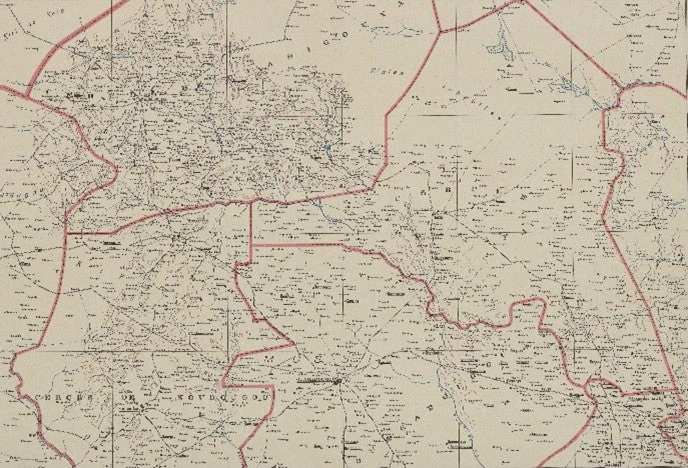
Figure 1: Raw Map
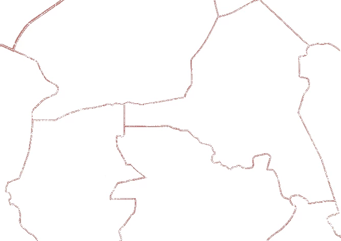
Figure 2: Map after Extracting Red Border
Georeferencing
Once you have your map with the extracted features, you now need to precisely situate the resulting image onto a current map. This step is referred to as georeferencing, and it is crucial but not always straightforward. Historical maps are not accurately drawn, and often the same landmarks, cities or even natural features may not exist on the more contemporary map. Some maps already come with coordinate grid information, while for others, one may need to manually locate the points that exist both on the old and on the recent map. Covering all the intricacies of georeferencing requires a post of its own; you should in particular read up on the transformation setting that is best suited to your map. In this example, I used the ‘georeferencer’ plugin in QGIS and the nearest neighbour transformation to situate my historical map onto OpenStreetMap.
Contouring and Buffering
Once you have georefenced your map, it exists in QGIS as a raster image. You now need to convert the raster image into a vector shapefile to increase the usability of the data. In her paper, Anna Peichel suggests the use of the GDAL contour tool in QGIS to achieve this. Although it has more sophisticated uses, what it basically does for us here is to trace the boundaries of each group of pixels within our raster image and convert it into data points. The main setting is the ‘interval between contour lines’, which may increase or decrease the number of elements that are contoured. It is therefore essential for you to see what interval works best for your analysis (here I used the interval of 50). Since the objective is to get one singular line for the border and not multiple data points, we can then use the QGIS buffering tool to merge various contours into one. The setting to keep in mind here is ‘distance’, which dictates the thickness of the buffer (here I choose 0.01 degrees). It is also important to check the ‘dissolve result’ option to ensure that we get one homogenous buffer.
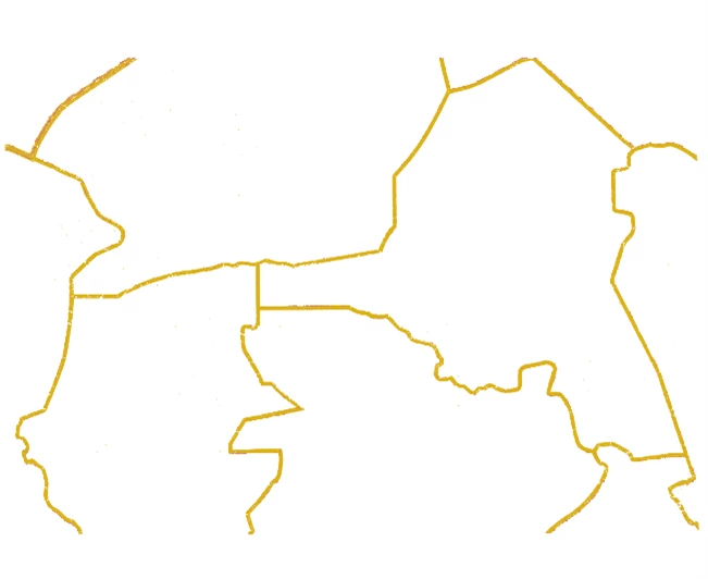
Figure 3: Map after Contouring
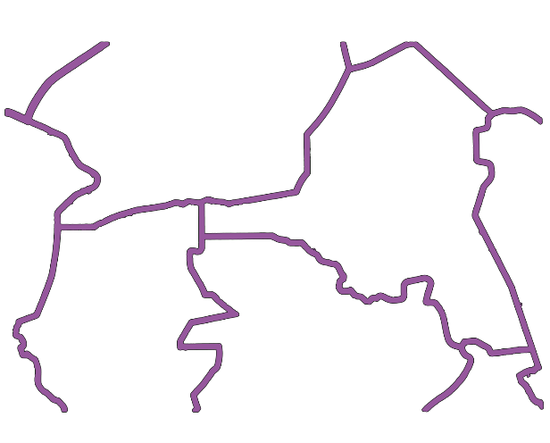
Figure 4: Map after Buffering
Skeletonizing
For the last step, all you need to do is to extract the centerline of your buffer, which gives you a multipoint shapefile that can be used as the border for your analysis. Both Anna Piechl and I are unable to find a satisfying tool in QGIS (though some Python tools may exist), so we use the ‘skeletonize’ feature of the GIS software OpenJump. The main setting of interest here is the ‘minimum number of forks’ that determines how many secondary outgrowths emerge along with the main centerline (6000 worked best for me). Once you run this algorithm and import the shapefile back into QGIS, you should be able to see the final output as one line that forms the border of interest. If you find that the output has secondary lines that are not part of the original border, it is always possible to manually edit the shapefile to get rid of any errors. If you wish to have polygons (for example to treat one administrative unit as one data point) rather than lines, you can use the ‘vector geometry’ tool to transform the shapefile from multiline to polygon.
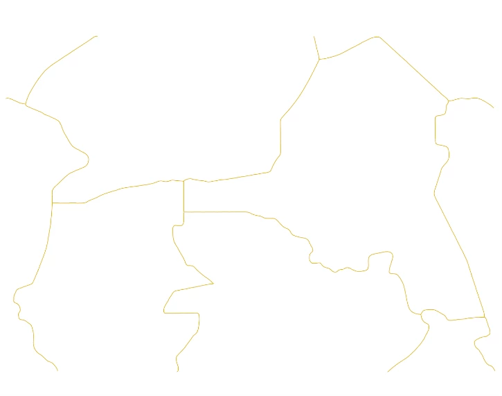
Figure 5: Final Boundary after Taking Centerline
Conclusion
These steps provide a method that can be used to increase precision when extracting historical boundaries, especially for researchers without extensive knowledge of GIS software. This process can work better than manually drawing the border especially when the border contains lines that are not straight. This is because GIS softwares like QGIS do not provide a straightforward methodology to draw curved lines. Semi-automatizing boundaries (as opposed to manual extraction) can also help in increasing the replicability of results. However, as in all research, it is important to remember that there is no one-size-fits-all solution. It is necessary to assess the costs and benefits of this approach compared with other alternatives depending on the research question and its specific requirements.
I would like to thank Camille Falezan (MIT) and Shirley Cheng (Stanford) for their help in exploring this methodology.
Vrinda Sharma is a consultant at the Africa Gender Innovation Lab of the World Bank and a PhD student at the Paris School of Economics. Twitter: @VSharma2211

Join the Conversation