A couple of months ago, I wrote about a new metric to assess heterogeneous treatment effects (HTE) that allows you to see, visually, if there are HTE in your study or not. One of the nice things about our blog, after more than 11 years, is that people do try out some of the proposed new methods in our posts. Further, a subset of them write to us with follow-up questions or updates. Today, I report some useful follow-up evidence from two studies that quickly tried to apply the metrics proposed in that post.
Borrowing from the previous post to quickly summarize the issue at hand, a new package in R introduced a new function called rank_average_treatment_effect, which estimates a rank-weighted ATE, or RATE, in grf. This is based on a paper by Yadlowsky et al. (2021). Once you estimate your conditional ATEs, or CATEs, you can feed them into the function and estimate what the authors call the Targeting Operator Characteristic, which is a curve comparing the benefit of treating only a certain fraction q of units to the overall average treatment effect. If there are HTEs, the curve will start high for the individuals with the highest expected benefit and declines until it equal ATE when q=1, i.e., everyone is included. This is nice because the area under this curve gives an immediate sense of whether there are HTE in the data or not: if the estimated targeting rule does well in identifying HTE, we’d expect the area under the curve to be a large number. If it does not do so well or there are no HTE, the same figure could be close to zero.
As the tutorial on RATE concludes, if you have a graph that suggests not much is going on, it could be “…attributed to a) low power, as perhaps the sample size is not large enough to detect HTEs, b) that the HTE estimator does not detect them, or c) the heterogeneity in the treatment effects along observable predictor variables are negligible.” In this update, I want to focus on signs that suggest that perhaps the power is low, or the estimator is not doing a good job of detecting HTE.
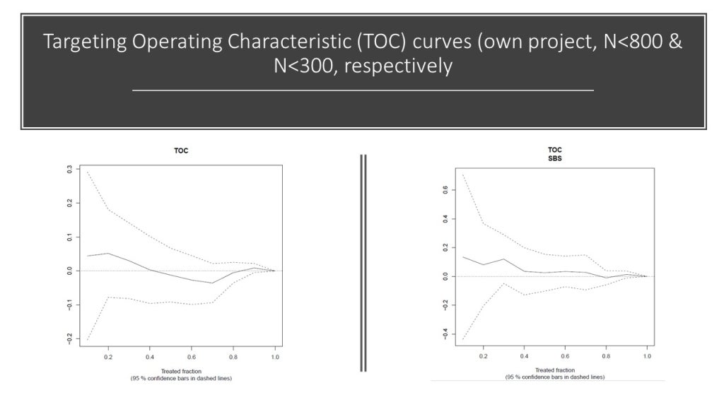
In our own work, we got curves like the ones you see below. The sample size on the left, for the whole sample is about 800 and it is lower for a sub-sample on the right. You can see that, the TOC would ideally decline monotonically, but it does not in these graphs. The reason is sampling variation or low signal: because of split sampling and estimating CATE in one sample and evaluating it in another one, the average treatment effect in a high quintile may turn out to be worse than in a low quintile. It is evidence that your CATE model is poorly calibrated. My co-author, looking at these at the time, very astutely wondered if this analysis would work better in a follow-on paper that pools all the data from the different phases of our experiment…
Around the same time, colleagues (Manisha Shah, Sarah Baird, Jennifer Seager, Benjamin Avuwadah, and Joan Hamory) working on a three-country study looking at the impact of adolescent girls’ life skills program on mental health outcomes and wanting to assess HTE by country, showed me their graphs, with the same problems. In their multi-site, clustered RCT (from GAGE), the average sample size is 1,500 and the average number of clusters is about 100 (both with some variation across the three countries). As you can see below, their curves for each country also zig zag instead of showing a smooth decline.

So, this suggests that even nicely powered field RCTs may not be able to use these methods successfully to assess HTEs in their contexts. Or, perhaps, there is really not a lot going on with respect to HTEs in these studies. But there is a nice ending to the story, perhaps a glimmer of hope. The authors of the study persisted and thought that maybe they want to pool all the data and examine heterogeneity that way:
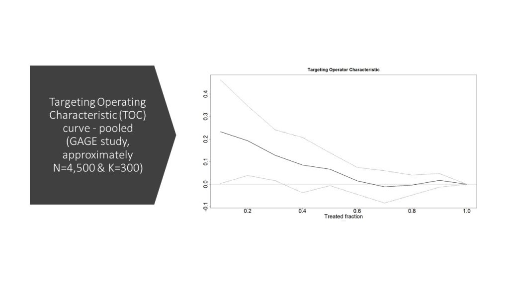
Voilà! In this graph, there is evidence that there are HTEs – with about 0.2 SD effects for the top 20% in CATE compared with no effect of the program for the bottom 40% of the CATE distribution. Furthermore, the curve nicely slopes downwards for most of the range, with tiny blips up and down in the bottom quartile.
While the evidence presented here is not proof that statistical power is the main underlying issue, it is suggestive. The lesson that I take away for the typical field RCT in development economics is that these new methods are worth trying, as the cost is low. However, you might often get equivocal results suggesting no HTE, whereas it might simply be that it’s there and meaningful but you’re not able to detect it. Individually randomized trials that have large N will have a better chance than the typical clustered RCT with 100 clusters and about 1,000-2,000 observations.

Join the Conversation