I think one of the first times I ever heard of the inverse hyperbolic sine (or asinh() in Stata) was in a blog post by Chris Blattman in 2011, which in turn linked to a Frances Woolley blogpost. The I.H.S. transformation was pitched as a solution to the problem one faces when wanting to take logs, but where there are zeros (or sometimes also negative values) in the data. Instead of the kludge ln(y+1) which no one was happy with, the recommendation was instead to use asinh(y) = ln(y+(y2+1)1/2), which Woolley wrote “can be interpreted in exactly the same way as a standard logarithmic dependent variable. For example, if the coefficient on "urban" is 0.1, that tells us that urbanites have approximately 10 percent higher wealth than non-urban people.”. Blattman even claimed it was David Card-approved. Many people (including myself) jumped at the chance to use this approach given the common existence of zeros in outcomes like income and profit. A 2020 OBES paper by Bellemare and Wichman discussed how to interpret elasticities in different I.H.S. models, and the fact this paper has already accumulated over 750 citations shows how popular this transform has become.
The shine comes off the (i.h.) sine
However, several recent papers have raised concerns about this transform, and particularly about how to interpret the magnitude of treatment effects estimated for an i.h.s. outcome.
First, papers by de Brauw and Herskowitz, and Aihounton and Henningsen note that the estimated coefficients and resulting elasticities can be quite sensitive to the units that the outcome is measured in. For example, if income is measured in Rupees versus thousands of Rupees versus millions of Rupees, the estimated percentage increase in earnings from program participation can vary. Aihounton and Henningsen then essentially view this as a robustness and data fitting problem, with the solution of repeating the regression with different units of measurement, seeing how sensitive the results are, and using a criteria like the R2 to choose which units of measurement to prefer. Bellemare and Wichman take a somewhat similar approach, arguing that one should choose units so that the untransformed means are greater than 10 (e.g. use dollars, not thousands of dollars for monthly income as an outcome), so that elasticities are somewhat stable.
However, new working papers by Mullahy and Norton, and Chen and Roth highlight and emphasize an issue that arises when the data have a mass of zeros – which is often the main reason people are wanting to use this transform in the first place. The issue is that the estimated i.h.s. treatment effect reflects a combination of both the extensive margin effect (how many units change from zero to a positive value), and the intensive margin effect (what the percent increase is from treatment for those with positive values) – with different choices of units for y changing how much weight is put on one versus the other. To see, this consider this graph from Figure 2 in Aihounton and Henningsen, which shows the distribution of earnings in 1978 of participants in the famous national supported work experiment used by Lalonde and many others after him.
Figure 2 from Aihounton and Henningsen, showing how shape of i.h.s. distribution depends on units
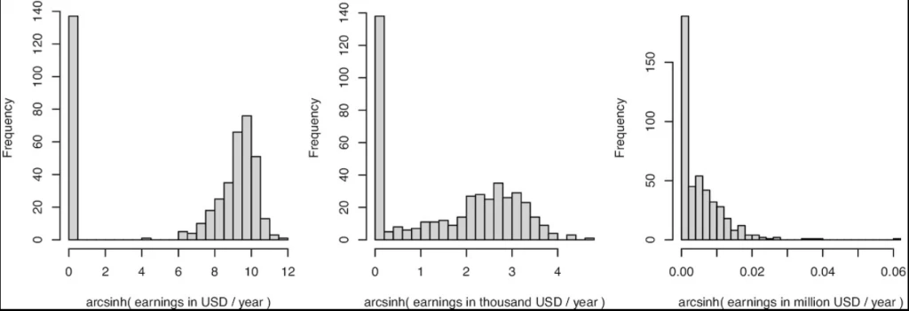
· On the left, when earnings are measured in USD per year, the i.h.s. transformation separates the zeros from the positive values. Here the distribution starts to look like a binary distribution – you either have zero income or positive income, and if treatment causes people to move from zero to a positive value, the i.h.s. model will mostly capture the linear probability model extensive margin effect. Chen and Roth note that if one follows the Bellemare and Wichman recommendation of re-scaling the units so that the mean of y is large, this is what one will typically end up with.
· On the right, when earnings are measured in millions of USD per year, there is no discernable separation between the zeros and other values, and the i.h.s. transformation will then essentially operate like running a linear regression of the untransformed y in levels – capturing mostly the intensive margin effect.
· The transformation in the center, will give you something in between – where the estimated effect will be more of a mix of the extensive margin and intensive margin effects.
(Addendum: see also this working paper by Delius and Sterck for another example, and for discussion of the case of negative values).
So with the exact same data set, when there are a bunch of zeros and action on the extensive margin, different choices of units can give very different coefficients, which is a problem if you want to interpret these coefficients as percentages. Moreover, it can also make a difference for whether the estimated effects are statistically significant –e.g. Chen and Roth show the t-stat will also converge to that of the t-stat of the extensive margin estimate when y is expressed in units that make it large.
Chen and Roth re-estimate 10 papers published in the AER that used the i.h.s transformation for at least one outcome, and illustrate how re-scaling the outcome units by 100 can lead to a change of more than 100% in the estimated treatment effect – with the largest changes coming for programs that had impacts on the extensive margin. E.g. In Rogall (2021)’s work on the Rwandan genocide, he looks at how the presence of armed groups fosters civilian participation in the violence. The extensive margin effect is 0.195, so a big extensive margin change. The estimated treatment effect then changes from 1.248 to 2.15 depending on whether y or 100*y is used as the outcome – which implies a massive change in the implied percentage change effect if interpreting these as either log points or like a log variable.
Yikes, so should we just give up on using the i.h.s?
These issues should make one a lot more cautious about using, and especially about interpreting, the i.h.s. transform. But whether, and how, to replace it depends on why you are doing it in the first place, and on what suitable alternatives are available. Afterall, the reason people starting using this was because of dissatisfaction with some existing approaches like dropping the zeros or using log(y+1).
First the bad news. Chen and Roth show that when there are zero-valued outcomes, there is no treatment effect parameter that satisfies all three of the following desirable properties: (i) it is an average of individual-level treatment effects; (ii) it is invariant to the scaling of outcomes; and (iii) it is point-identified from the marginal distributions of the potential outcomes. So there is no single optimal alternative method, but rather you need to give up at least one of these assumptions, and how to do so will depend on context and what you care about.
Here are (my interpretations of) some suggested approaches from Chen and Roth:
1. If there are few zeros/a very small extensive margin effect – then Lee bounds may be the answer: the issues are all arising because of the zeros and movement at the extensive margin from zero to a positive value. But if there are not very many zeros, or very little movement at the extensive margin, then one could relax point identification and get quite narrow Lee bounds on the intensive margin effect of the ATE of log(y), or asinh(y). Note that this requires fewer assumptions when there are not many zeros, whereas when there are a lot of zeros and just no treatment effect on the extensive margin, one needs to assume that treatment does not change the selection of who ends up at 0. This is akin to the monotonicity assumption of Lee. E.g. suppose treatment increases labor force participation by 2 percentage points- one needs to assume that everyone who doesn’t work in treatment would have also not worked in control.
2. Can you redefine the outcome and then estimate the treatment effect in levels to get something that is still interpretable? There are two main reasons I see applied researchers using the i.h.s. transformation – to get an outcome they can interpret as a percent change, and as a statistical tool to deal with highly skewed outcomes that also have zeros. If the issue is just interpretation as a percentage, then one approach is to estimate the model in levels, and then communicate treatment effects as a percent of the control mean – as researchers often do. Or rather than estimating the level effect on y, one could estimate the level impact on y/x for some normalizing value of interest x. E.g. perhaps you are estimating treatment effects of a program on income, and the problem is that everyone is unemployed to start with, so baseline income is zero. One could use other data to run a model that predicts income given pre-treatment individual characteristics, and then the outcome of interest could be redefined as the ratio of realized income to predicted income. In practice I would worry this may just put in more noise though. Or if the issue is the statistical reason, rather than using asinh(y), one can examine treatment effects on a winsorized value of y, or on e.g. outcomes such as a binary value for y exceeding some threshold such as a poverty line.
3. Redefine the estimand, so it is no longer an average of individual-level treatment effects: using quantile treatment effects is one approach here.
4. Explicitly take a stand on how much you value the extensive versus intensive margin effects. For example, you/a policymaker might decide that you value getting someone to move from earning 0 to earning $100/month as worth the same as getting an employed person to earn 25% higher income. Then, if y is measured in 100s of dollars, you could set use a transform of m(y) = log(y) for y>0, and m(0) = -0.25. In practice it may be hard to get agreement on this trade-off, but this calculation at least makes it explicit.
5. Estimate the i.h.s., but don’t interpret this as a percentage change. In discussing this with Jon Roth, he noted to me the lesson should not be to examine sensitivity to multiplying the units by 10 or 100, and then saying we are ok if they don’t change much – if there is any extensive margin effect, then by changing the units enough, one can get pretty much any answer you want, since a percentage effect is not well-defined when there is an extensive margin. So then if one runs a regression on asinh(monthly profits in dollars), and gets a coefficient of 0.15, then rather than claiming there is a 15% increase in profits (a number which can change if we change the units), this should instead just be interpreted as the treatment impact on the inverse hyperbolic sine of monthly profits in dollars. Not the easiest thing to explain to a policymaker, but if you want to use the asinh() transformation because of highly skewed data and zeros and dissatisfaction with the other options above, then this is at least an accurate way of interpreting the results.
So while this recent work is perhaps not quite the death knell of the i.h.s. transform, it does show that it really does not magically solve the issues that prevented us from using log(y), and that interpreting the magnitudes of treatment effects on i.h.s. outcome as percentages will often be fraught with peril. In practice, researchers will often estimate impacts on the extensive margin, some sort of winsorized levels, and then perhaps an i.h.s. or log transform, as well as maybe quantile effects. These papers highlight the importance of documenting how many zeros are in the data, how big the extensive effect is, and thinking careful about how to value extensive versus intensive margin effects.

Join the Conversation