For quite a few reasons, many researchers have become increasingly skeptical of a lot of attempts to use instrumental variables for causal estimation. However, one type of instrument that has enjoyed a surge in popularity is what is known as the “judge leniency” design. It has particularly caught my attention recently through a couple of applications where the judges are not actually court judges, and it seems like there could be quite a few other applications out there. I therefore thought I’d summarize this design, these recent applications, and key things to watch out for.
The basic judge leniency set-up.
This design appears to have gained first prominence through studies which look at the impact of different types of experience with the criminal legal system. A classic example is Kling (2006, AER), who wants to look at the impact of incarceration length (S) on subsequent labor outcomes (Y). That is, he would like to estimate an equation like:
Y(i) = a + bS(i) + c’X(i)+ e(i)
The concern, of course, is that even controlling for observable differences X(i), people who get longer prison sentences might be different from those who get given shorter sentences, in ways that matter for future labor earnings.
A solution comes from the fact that assignment of cases to judges is randomly assigned, conditional on the date and location of case filing. Then a key observation is that some judges appear to be systematically harsher at sentencing than others. So letting Z be a vector of dummies for judges, a first stage can be estimated by:
S(i) = f + g’Z(i) + h’D(i) + w(i)
Where D(i) are a set of controls for the things judge assignment is conditional on (e.g. date, location). A key point to note here is that each judge is an instrument, and so one needs to worry about concerns about weak instruments (e.g. Kling has 52 different judge dummies as the instruments). The approach has then been to use a leave-one-out jackknife IV (JIVE) approach.
Subsequent papers appear to have moved away from directly including dummies for each judge to using a more aggregated residualized judge leniency measure as the instrument. For example, Dahl, Kostøl and Mogstad (2014, QJE) use Norwegian data to look at how participation in disability insurance by parents affects subsequent participation in welfare by their children. They use random assignment of judges to disability insurance applicants whose cases were initially denied. They then define a judge leniency measure as the share of appeals allowed by a judge on all other cases apart from the one being considered, call this A(-i). They then regress this tendency on being generous or strict with appeals on year*department dummies to account for randomization occurring within these pools, and use the residualized leniency as the instrument. This approach is also followed by Dobbie, Goldin and Yang (2018, AER) who use differences in the tendencies of bail judges to estimate the causal impact of pre-trial detention on subsequent defendant outcomes.
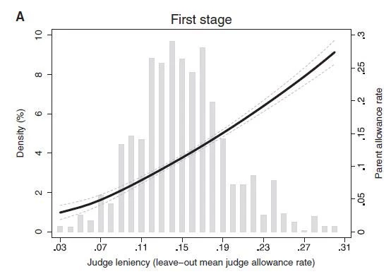
One nice feature of this residualized leniency approach is that it becomes easy to visually show where the variation in the first-stage is coming from. Figure 1 below shows both a histogram of these judge leniency rates, showing that there is quite a wide variation in leniency, with a generous judge (at the 90th percentile) approving 22% of appeal cases, whereas a strict judge (at the 10th percentile) approves only 9 percent (X-axis). This is the instrument, and the fitted local linear line shows this translates approximately linearly into predicting the first-stage of whether parents are on disability insurance.
Figure 1: Example of a first-stage in a leniency design (Dahl et al, 2014).
Moving beyond court judges to use this strategy with other capricious decision-making
I hadn’t thought this strategy would have many uses outside of studies on crime, but several recent papers have got me to think that this method may be more applicable than I had originally thought. Some examples of using this approach outside of court judges are:
- Doyle et al. (2015, JPE), who want to look at whether more expensive hospitals improve patient outcomes. They use the idea that ambulance companies are pseudo-randomly assigned to patients in an emergency, and different ambulance companies have different tendencies to favor particular types of hospitals.
- Farre-Mensa, Hegde and Ljungqvist have a recent working paper that aims to measure the value of patents to startups by leveraging the quasi-random assignment of patent applications to examiners with different propensities to grant patents. Moving from an examiner at the 25th percentile to one at the 75th percentile would increase a startup’s probability of being granted a patent by 11.8 percentage points.
- A new paper by Juanita Gonzalez-Uribe and Santiago Reyes was what really got me thinking about this type of design more. They want to look at the impacts of a Colombian business accelerator, for which applicants were selected based on the average score from three randomly chosen judges. They show moving from moving from the bottom to the top quartile of scoring generosity roughly doubles acceptance rates into the accelerator.
Caveats and Lessons for Implementation
This all sounds great, but before you run out to search for capricious decision-making, here are some points to consider.
- What is the assignment mechanism? Some of the studies have actual random assignment of judges to cases, or scorers to tests. Others call it “quasi-random”, which basically means decision-makers are assigned to individual cases in a way that doesn’t seem like it should be related to outcomes, but is not completely random. But you really want to know all the details here – e.g. Dobbie, Goldin and Yang note that bail hearings following driving under the influence arrests tend to occur more in the evenings and weekends, so if certain judges are more likely to work these shifts, simple leave-one-out means will still be biased – and so they control for time and day effects. Likewise, you want to know if randomization is at the individual case/test level, versus for batches (i.e. is it individual or clustered random assignment), and account for this accordingly.
- Does the exclusion restriction hold? Even with random assignment of judges/scorers, the exclusion restriction here is that the type of judge you are assigned only affects the outcomes through one specific measure (e.g. incarceration length, getting a patent, getting accepted to the accelerator). But judges may do other things that independently affect outcomes – e.g. in court, judges may say things that change defendant’s beliefs and attitudes, they may impose other conditions on defendants apart from incarceration length or bail decision, etc.); judges of entrepreneur pitches may give feedback on proposals that independently affect outcomes apart from through the score. The exclusion restriction seems easier to justify when there is no interaction between the decision-maker and case being decided (e.g. scorers marking anonymous essays).
- Being clear what effect this design will identify: if there is treatment effect heterogeneity, the IV estimator here will deliver a weighted average of marginal treatment effects that may be hard to interpret. If one is prepared to assume monotonicity, then it will deliver the LATE – the impact for people whose status is affected by whether they get a stricter or more generous judge. E.g. for defendant’s whose incarceration length is affected by which judge they get, or business accelerator applicants who are marginal enough that whether or not they get accepted depends on whether they get a score boost from a generous judge or score penalty from a stricter judge. Monotonicity assumes that judges are just uniformly more or less generous. As Dobbie et al. note in their case, this “requires that individuals released by a strict judge would also be released by a more lenient judge, and that individuals detained by a lenient judge would also be detained by a stricter judge”.
Figure 2: Monotonicity Maybe Not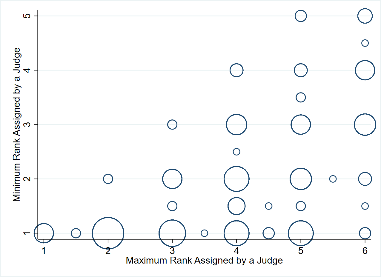
This seems a more generalizable lesson – judges/scorers are likely to differ not just in generosity, but also in preferences – e.g. in courts, some judges may be harsher on certain types of defendants or certain types of crimes; scorers marking essays may differ in how much they value style vs substance; judges of business plans may find different ideas appealing etc. So I suspect it will be rare for monotonicity to hold in most cases, and so this method will likely not yield a well-defined LATE.
Further reading:
- Peter Hull has a 1-page note that makes the point that the true dimensionality of the instrument is still the number of judges, even if one uses a residualized or jackknife approach. The consequence is that researchers run the risk of greatly overstating their first-stage F-statistics when using constructed instruments (the residualized approach) and treating this as if they only have a single instrument instead of many.
- Coincidentally, just after I finished writing this post, Seema Jayachandran published a NY Times Economic View column that summarizes the results of two studies of cash bail that use this judge leniency identification method (including the Dobbie et al. one I mention above).

Join the Conversation