Updated September 14, 2020 to reflect that my initial post using an older version of rwolf, and that a new version of wyoung that allows for multiple treatments has been released. And updated again April 16, 2021 to reflect a new update to wyoung which allows for more easily including different controls in each equation.
There are a growing number of user-written Stata packages for conducting multiple hypothesis testing. I thought I would compare the pros and cons of several of these, both as a way of helping remind myself of which packages work for which settings, as well as to potentially help others. I start by acknowledging gratitude to the authors of these various packages for writing this code at all, so even when I complain that it doesn’t do everything I need in particular applications, it may be very useful for other needs.
What is the problem we are trying to solve?
Suppose we have run an experiment with four treatments (treat1, treat2, treat3, treat4), and are interested in examining impacts on a range of outcomes (y1, y2, y3, y4, y5). We run the following treatment regressions for outcome j at time t:
Y(j,t) = a + b1*treat1+b2*treat2+b3*treat3+b4*treat4 + c1*y(j,0) + d’X + e(j,t)
With 5 outcomes and 4 treatments, we have 20 hypothesis tests and thus 20 p-values. Here’s an example from a recent experiment of mine (where the outcomes are firm survival, and four types of business practice measures) and the treatments are different ways of helping firms learn new practices – where the p-values are shown under the coefficients.
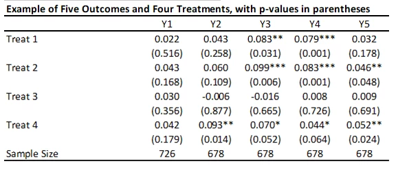
Suppose that none of the treatments have any effect on any outcome (all null hypotheses are true), and that the outcomes are independent. Then if we just test the hypotheses one by one, then the probability that of one or more false rejections when using a critical value of 0.05 is 1-0.95^20 = 64% (and using a critical value of 0.10 is 88%. As a result, in order to reduce the likelihood of these false rejections, we want some way of adjusting for the fact that we are testing multiple hypotheses. That is what these different methods do.
Anderson’s code for FDR sharpened q-values
One of the most popular ways to deal with this issue is to use Michael Anderson’s code to compute sharpened False Discovery Rate (FDR) q-values. The FDR is the expected proportion of rejections that are type I errors (false rejections). Anderson discusses this procedure here.
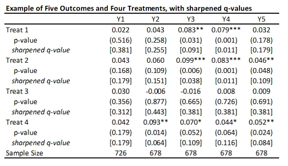
This code is very easy to use. You need to just save the p-values and then read them as data into Stata, and run his code to get the sharpened q-values. For my little example, they are shown in the table below.
A few points to note:
· A key reason for the popularity of this approach (in addition to its simplicity) is seen in the comparison of the original p-values to sharpened q-values. If we were to apply a Bonferroni adjustment, we would multiply the p-values by the number of outcomes (20) and then cap at 1.000. Then, for example, the p-value of 0.031 for outcome Y3 and treatment 1 would be adjusted to 0.62. Instead the sharpened q-value is 0.091. That is, this approach has a lot greater power than many other methods.
· Because this takes the p-values as inputs, you have a lot of flexibility into what goes into each treatment regression: for example, you can have some regressions with clustered errors and some without, some with controls and some without, etc.
· As Anderson notes in his code, sharpened q-values can actually be LESS than unadjusted p-values in some cases when many hypotheses are rejected, because if there are many true rejections, you can tolerate several false rejections too and still maintain the false discovery rate low. We see an example of this for outcome Y1 and treatment 1 here.
· A drawback of this method is that it does not account for any correlations among the p-values. For example, in my application, if a treatment improves business practices Y2, then we might think it is likely to have improved business practices Y3, Y4, and Y5. Anderson notes that in simulations the method seems to also work well with positively dependent p-values, but if the p-values have negative correlations, a more conservative approach is needed.
mhtexp
This code implements a procedure set out by John List, Azeem Shaikh and Yang Xu (2016), and can be obtained by typing ssc install mhtexp
This procedure aims to control the familywise error rate (FWER), which is the probability of making any type I error. It builds on work by Romano and Wolf, and uses a bootstrapping approach to incorporate information about the joint dependence structure of the different tests – that is, it allows for the p-values to be correlated.
· This command allows for multiple outcomes and multiple treatments, but does not allow for the inclusion of control variables (so no controlling for baseline values of the outcome of interest, or for randomization strata fixed effects), and does not allow for clustering of standard errors.
· The command is then straightforward. Here I have created a variable treatgroup which takes value 0 for the control group, 1 for treat 1, 2 for treat 2, 3 for treat 3, and 4 for treat 4. Then the command is:
mhtexp y1 y2 y3 y4 y5, treatment(treatgroup) bootstrap(3000)
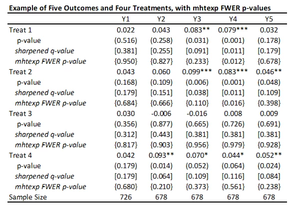
I’ve added these FWER p-values to the table below. While not as large as Bonferroni p-values would be, you can see they are much larger that the original p-values and sharpened q-values. Not much of this is due to not including the control variables in this particular case, since the raw p-values don’t change that much with the addition of the controls. Instead, this reflects the issue of using FWER with many comparisons – in order to avoid making any type I error, the adjustments become increasingly severe as you add more and more outcomes or treatments. That is, power becomes low. In contrast, the FDR approach is willing to accept some type I error in exchange for more power. Which is more suitable depends on how costly false rejections are versus power to examine particular effects.
rwolf
Note my original post used an earlier version of this command which allowed only a single treatment. The command now allows for multiple treatments.
This command calculates Romano-Wolf stepdown adjusted p-values, which control the FWER and allows for dependence among p-values by bootstrap resampling. It is therefore aiming to do the same things as mhtexp, although with a slightly different algorithm, and was developed by Romano and Wolf themselves (along with Damien Clarke), and is described here. To get this type ssc install rwolf
· In contrast to mhtexp, this command does allow for you to include control variables in the regression, but does force them to be the same for every outcome. It also has an option to include the baseline value of the outcome, so you can allow this to differ across outcomes and do Ancova (so long as you don't have missing baseline values and need a separate dummy for a missing baseline).
· It also allows for clustered randomization, and can do the bootstrap re-sampling by taking account of both randomization strata and of clustered assignment.
An earlier version of the command only allowed for a single treatment, but now the command allows for multiple treatments. However, it currently only runs the multiple testing correction for each treatment at a time. That is, it will correct for testing treat1 on 5 outcomes, but not for the fact that you are also testing other treatments at the same time. As such, I currently do not recommend its use for multiple treatment corrections. This will get addressed in a future update, and I will aim to revise this post then.
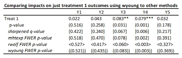
· To illustrate for a single treatment, I will just keep treatment 1 and the control, and then also compare the other methods above when applied just to this set of 5 comparisons (treatment 1 effects on each of the five outcomes). Then the command is:
rwolf y1 y2 y3 y4 y5 if treatment<=1, indepvar(treat1) controls(i.strata) reps(1000)
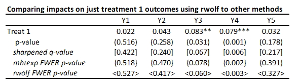
You can see the rwolf p-values are pretty similar to those from mhtexp as expected.
With multiple treatments, you can use code like: rwolf y1 y2 y3 y4 y5, indepvar(treat1 treat2 treat3 treat4) reps(1000) method(areg) abs(batchno) bl(_bl) strata(batchno) seed(456) r - but see note above, I do not recommend using the command for multiple treatment corrections at the moment, since it only adjusts within a treatment, and not across treatments.
The command also now allows you to use commands like areg, ivreg, etc. so long as you are using the same method for all regressions.
wyoung
This command, programmed by Julian Reif, calculates Westfall-Young stepdown adjusted p-values, which also control the FWER and allow for dependence amongst p-values. This method is a precursor to the Romano-Wolf procedure, using bootstrap resampling to allow for dependence across outcomes. Romano and Wolf note that the Westfall-Young procedure requires an additional assumption of subset pivotality, which can be violated in certain settings, and so the Romano-Wolf procedure is more general. I don’t have a great sense of when it breaks down.
To get this command, type ssc install wyoung
Update April 2021: use the command below instead
net install wyoung, from("https://raw.githubusercontent.com/reifjulian/wyoung/controls-option") replace
· A nice feature of this command is that it allows you to have different control variables in different equations. So you can control for the baseline variable of each outcome, for example. It also allows for clustered randomization and can do bootstrap re-sampling that accounts for both randomization strata and clustered assignment.
· When I first blogged about these commands, it it only allowed for a single treatment variable.
Like the Romano-Wolf example above, I therefore look at this adjustment on the five outcomes for treatment 1, and compare to the other methods. The command is a bit longer looking, because it allows for different regressions – note I have no baseline outcome for y1 (survival) since all firms were alive to begin with, and then control for the baselines levels of the other outcomes b_y1, etc.
wyoung, cmd("areg y1 treat1, r a(strata)" "areg y2 treat1 b_y2, r a(strata)" "areg y3 treat1 b_y3, r a(strata)" "areg y4 treat1 b_y4, r a(strata)" "areg y5 treat1 b_y5, r a(strata)" familyp(treat1) bootstraps(1000) seed(124)
This gives pretty similar adjusted values as mhtexp and rwolf, which is to be expected since they are all trying to control the FWER using similar approaches.
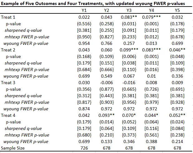
After the update, the command now allows for multiple treatments. When you have the same controls across all regressions, the command is quite simple:
wyoung y1 y2 y3 y4 y5, cmd(areg OUTCOMEVAR treat1 treat2 treat3 treat4, r a(strata)) familyp(treat1 treat2 treat3 treat4) bootstraps(1000) seed(123)
If you have different controls in each equation, then the command is a lot more clunky - you have to list each equation the number of times it is being tested, and each variable for each equation. e.g.
wyoung, cmd("areg y1 treat treat2 treat3 treat, r a(batchno)" "areg y2 treat1 treat2 treat3 treat4 basey2, r a(batchno)" "areg y3 treat1 treat2 treat3 treat4 basey3, r a(batchno)" "y4 treat1 treat2 treat3 treat4 basey4, r a(batchno)" "y5 treat1 treat2 treat3 treat4 basey5, r a(batchno)" "areg y1 treat treat2 treat3 treat, r a(batchno)" "areg y2 treat1 treat2 treat3 treat4 basey2, r a(batchno)" "areg y3 treat1 treat2 treat3 treat4 basey3, r a(batchno)" "y4 treat1 treat2 treat3 treat4 basey4, r a(batchno)" "y5 treat1 treat2 treat3 treat4 basey5, r a(batchno)" "areg y1 treat treat2 treat3 treat, r a(batchno)" "areg y2 treat1 treat2 treat3 treat4 basey2, r a(batchno)" "areg y3 treat1 treat2 treat3 treat4 basey3, r a(batchno)" "y4 treat1 treat2 treat3 treat4 basey4, r a(batchno)" "y5 treat1 treat2 treat3 treat4 basey5, r a(batchno)" "areg y1 treat treat2 treat3 treat, r a(batchno)" "areg y2 treat1 treat2 treat3 treat4 basey2, r a(batchno)" "areg y3 treat1 treat2 treat3 treat4 basey3, r a(batchno)" "y4 treat1 treat2 treat3 treat4 basey4, r a(batchno)" "y5 treat1 treat2 treat3 treat4 basey5, r a(batchno)") familyp(treat1 treat1 treat1 treat1 treat1 treat2 treat2 treat2 treat2 treat2 treat3 treat3 treat3 treat3 treat3 treat4treat4 treat4 treat4 treat4) bootstraps(1000) seed(124)
Update April 14, 2021: Julian has added a new option to make it much easier to include different controls in each equation, and the syntax is much simpler as a result:
wyoung Y1 Y2 Y3 Y4 Y5, cmd(areg OUTCOMEVAR treat1 treat2 treat3 treat4 CONTROLVARS, r a(strata)) familyp(treat1 treat2 treat3 treat4) controls("constant" "b_Y2" "b_Y3" "b_Y4" "b_Y5") bootstraps(1000) seed(123);
Note that since I did not want to include any controls for outcome Y1, I created a variable called constant which just has value one for everyone, and use that in the command.
This gives the adjusted FWER p-values in the table below, which differ from the mhtexp ones in using Westfall-Young rather than Romano-Wolf, and in controlling for baseline variables.
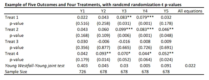
randcmd
This is a Stata command written by Alwyn Young that calculates randomization inference p-values, based on his recent QJE paper. It is doing something different to the above approaches. Rather than adjusting each individual p-value for multiple testing, it conducts a joint test of the sharp hypothesis that no treatment has any effect, and then uses the Westfall-Young approach to test this across equations. So in my example, it tests that there is no effect of any treatment on outcome Y1 (p=0.403), Y2 (p=0.0.045) etc., and then also tests the null of complete irrelevance – that no treatment had no effect on any outcome (p=0.022 here). The command is very flexible in allowing for each equation to have different controls, different samples, having clustered standard errors, etc. But it is testing a different hypothesis than the other approaches above.
Addendum: mhtreg
Turns out others have also realized these limitations, and Andreas Steinmayr has extended the mhtexp command to allow for the inclusion of different controls in different regressions, and for clustered randomization, with a command mhtreg
To get this: type
ssc install mhtreg
I tried this out, and it does indeed allow for different controls in different regressions. It is definitely an improvement on mhtexp. A couple of limitations to be aware of:
· The syntax is a bit awkward with multiple treatments – it only does corrections for the first regressor in each equation, so if you want to test for multiple treatments, you have to repeat the regression and change the order in which treatments are listed. E.g. to test the 20 different outcomes in my example, the code is:
mhtreg (y1 treat1 treat2 treat3 treat4 i.strata, r) (y1 treat2 treat3 treat4 treat1 i.strata, r) (y1 treat3 treat4 treat1 treat2 i.strata, r) (y1 treat4 treat1 treat2 treat 3 treat4 i.strata, r)
(y2 treat1 treat2 treat3 treat4 b_y2 i.strata, r) (y2 treat2 treat3 treat4 treat1 b_y2 i.strata, r)….
· It requires each treatment regression to actually be a regression – that is, to have used the reg command, and not commands like areg or reghdfe; or for you to be doing ivreg or probits, or something else – so you will need to add any fixed effects as regressors, and better be doing ITT and not TOT or other non-regression estimation. This can be contrasted with the wyoung command.
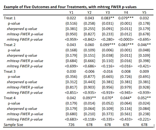
An additional thing to watch out for (that likely applies to the other commands as well) is that, even with the default 3000 bootstrap replications, the corrected p-values can change a bit from one random seed to another. This seems particularly an issue for really low p-values, where you are looking at uncommon events. For example, for outcome Y4, treatment 1, using three different seeds and mhtreg, I get adjusted p-values of 0.0003, 0.0057, and 0.011. So you may need to specify a lot more replications to get robustness of these adjusted values to choice of seed.
Here is the table of my results using mhtreg and comparing to the mhtexp and sharpened q-values. You see the results are similar to mhtexp, the differences are coming from the inclusion of baseline controls.
Putting it altogether
The table below compares the multiple hypothesis testing command continues. With a small number of hypothesis tests, controlling the FWER is useful, and then wyoung now seems to be the one I will prefer. With lots of outcomes and treatments, controlling the FDR seems the best approach, and so the Anderson q-value approach is my stand-by. I only wish it would account for correlations between outcomes. The Young omnibus test of overall significance is a useful compliment, but answers a different question.
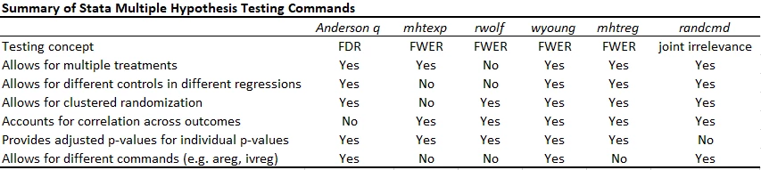
Note the updated version of rwolf does allow for multiple treatments (but only currently adjusts for testing multiple outcomes for a treatment, but not for multiple testing across treatments - so I do not recommend for multiple treatments), for different commands (areg, ivreg). You can include a different baseline variable in each regression, but otherwise need to have the controls be the same.

Join the Conversation