In my last post, I discussed testing for differential pre-trends in difference-in-difference studies. Suppose that we find that the pre-treatment trends of the treatment and control groups are different. Or that we are in a situation where power is low to detect important violations of parallel trends. Or we have a reason to think that some other shock in the economy may cause the post-treatment trends to differ, even if the pre-treatment trends were the same. For example, suppose we are looking at the impact of an employment program for youth, and the employment rate of the treated group was growing at 2% per month in the months before the intervention, whereas the employment rate of the control group was growing at only 1% a month, so the difference in trends is 1% per month. Parallel trends therefore does not hold. Can we still do DiD?
A new paper by Rambachan and Roth (2019) (Roth’s job market paper) addresses this issue. They note that one approach would be to assume that the pre-existing difference in trends persists, and to simply extrapolate this out. So in my employment example, we might assume that the difference in trends of 1% per month would continue to hold, so that if the control group has employment grow at 3% per month after the intervention, we would assume the treated group employment would have grown at 4% per month, and compare the actual employment rate to this counterfactual. This assumption is shown in the left-hand side of Figure 1 below, which assumes any pre-existing difference in trends precisely extrapolates. However, assuming the pre-treatment difference in trends carries out exactly is a very strong assumption, particularly if we did not have many pre-treatment periods over which to observe this. Rambachan and Roth suggest that researchers may instead want to consider robustness to some degree of deviation from this pre-existing trend, so that linear extrapolation need only be “approximately” correct, instead of exactly correct. In the right of Figure 1, this is realized by allowing the trend to deviate non-linearly from the pre-existing trend by an amount M – the bigger we make M, the more deviation from pre-existing trend.

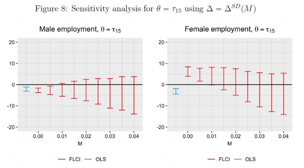
Then their paper shows that given M, we can identify a confidence set for the treatment parameter of interest – this is a partial identification approach. Researchers can then also find and report the breakdown point – how much of a deviation from the pre-existing difference in trends is needed before we can no longer reject the null. Figure 8 below, from their paper, illustrates how this works in practice. They consider the impact of a teacher collective bargaining reform on employment, in which parallel trends seem to hold for males, but in which there is a pre-existing negative trend for females. The left of the figure shows the DiD estimate for males in blue, a similar interval at M=0 in red (linear extrapolation of the pre-existing trend), and then intervals which get wider as we allow more and more of a deviation in trends. In contrast, for females, the DiD estimator in blue is of opposite sign to what would be obtained when we extrapolate the pre-existing trend at M=0, and then one sees how these results change as more deviations from these existing trends are allowed for.
Estimation involves solving a nested optimization problem, and so is not just a matter of plugging in different linear pre-trends into your OLS regression. The authors have written R code HonestDiD that will do this for you (and hopefully will write some Stata code in due course). Their paper also discusses how you can come up with reasonable benchmarks for what sort of deviation from parallel trends might be occur by using pre-trends, placebo groups, and economic theory; as well as other types of restrictions researchers may wish to impose on pre-trends, such as monotonicity. The implication is that you can now not just assert that parallel trends hold, but show how robust your results are to deviations from this assumption.
A second, related approach, is provided by Bilinski and Hatfield (2019). They recommend a move away from relying on traditional parallel trend pre-tests because of problems in both directions:
· If we fail to reject parallel trends, in many cases this is because power is low, as noted in the previous blog post.
· But if power is high, and we reject parallel trends, this doesn’t tell us much about the magnitude of the violation and whether it matters much for the results – with big enough samples, trivial differences in pre-trends will lead to rejection of parallel trends.
Instead, they propose a “one step up” model. The idea here is to first report treatment effect estimates from a DiD model with a more complex trend difference than you think to be the case – so if you think there are parallel trends, first estimate a model that allows for the two groups to have linear trends with different slopes by including a linear trend difference. Then compare this to the simpler model (e.g. which assumes parallel trends), and test whether the difference in treatment effects between the two models falls within some specified distance. A key issue here is determining what constitutes a “large’ difference – which takes you back to the type of graph shown above, which examines robustness to different degrees of deviation from parallel trends. The authors’ R code is under construction, and will be available here.
They note further that how much confidence we should have in the estimated treatment effects depends on how reliable extrapolation of the counterfactual will be. This is illustrated nicely in an application to examining the Affordable Care Act’s dependent coverage mandate. Suppose we have an event study plot like the "Any health insurance" plot on the left. The estimated treatment effect in the "usual" DiD model is 3%, while a model with a linear trend difference estimates a treatment effect of 1%. As these differ considerably, they consider a model with a more complex spline trend difference, which yields a larger treatment effect estimate of 4%. The spline model picks up on a divergence early in the pre-intervention period that flattened out. But if trends were only nearly parallel over the last portion of the pre-intervention period, we may not trust that they would have stayed that way in the post-period, over an equal or longer time horizon than they were parallel/slightly downward sloping in the pre-period. By contrast, in the "Dependent coverage" plot, models with a linear and spline trend differences are nearly identical, providing stronger evidence of a stable linear trend difference.

A third approach is proposed by Freyaldenhoven, Hansen and Shapiro (2019) in a recent AER paper. Their idea is a solution similar to instrumental variables to net out the violation of parallel trends. For example, suppose that one wants to look at the impact of a minimum wage change on youth employment. The concern is that states may increase minimum wages during good times, so that labor demand will cause the trajectory of youth employment to differ between treated and control areas, even without the effect of minimum wages. Their solution is to find a covariate (e.g. adult employment) which is also affected by the confounder (labor demand), but which is not affected by the policy (i.e. if you believe minimum wages don’t affect adult employment). Then this covariate can be used to reveal the dynamics of the confounding variable and adjust for it, giving the impact of the policy change. Importantly, this does NOT mean simply controlling for this covariate (which only works if the covariate is a very close proxy for the confounder of concern), but rather using it in a 2SLS or GMM estimator. I didn’t find the youth employment example overly convincing, but their paper provides other cases where this assumption may be more convincing: one example concerns the impact of SNAP program participation on household spending, where the main dataset has SNAP participation and the outcomes, and the concern is that income trends may determine both program participation and spending. Using a second dataset that has SNAP participation and income, they can instrument participation with leads of income, which requires assuming that households don’t reduce labor supply in anticipation of getting the program. Their Stata code is here.
Implications for applied work:
1. Rather than just asserting that parallel trends hold, or abandoning projects where a pre-test rejects parallel trends, these new papers focus on thinking carefully about what sort of violations of parallel trends are plausible, and examining robustness to these. Importantly, these methods should be used when there is reason to be skeptical of parallel trends ex ante, regardless of the outcome of a test of whether parallel trends hold pre-intervention. This type of sensitivity analysis will allow one to get bounds on likely treatment effects. A recent application comes from Manski and Pepper (2018), who look at how right-to-carry laws affect crime rates, obtaining bounds on the treatment effect under different assumptions about how much the change in crime rates in Virginia would have differed from those in Maryland in the absence of this policy change in Virginia.
2. Your default Difference-in-Difference estimation equation should allow for a linear trend difference. This is a key recommendation of Bilinski and Hatfield (2019).
3. Which approach to use to examine robustness will depend on how many pre-periods you have: with only a small number of pre-intervention periods, the Rambachan and Roth approach of bounding seems most applicable for sensitivity analysis; when you have more periods you can consider fitting different pre-trends as in Bilinski and Hatfield.
In a future post, I hope to return to my pile of DiD papers to discuss some of the other new developments that deal with issues such as heterogeneous treatment effects, multiple time periods, staggered timing of the policy changes, links to synthetic control methods, and more. Stay tuned. In the meantime, check out this summary page by Bret Zeldow and Laura Hatfield that offers their overview of many of the recent developments in DiD.

Join the Conversation