As our impact evaluations broaden to consider more and more possible outcomes of economic interventions (an extreme example being the 334 unique outcome variables considered by Casey et al. in their CDD evaluation) and increasingly investigate the channels of impact through subgroup heterogeneity analysis, the issue of multiple hypothesis testing is gaining increasing prominence.
One approach to dealing with multiple outcomes is to aggregate them into particular groupings to examine whether the overall impact of the treatment on a family of outcomes is different from zero. This is the approach a number of papers (including the Casey et al. one above) have used following O’Brien (1984) and Kling and Liebman (2004). This approach is useful if the intention is to see whether the global impact of a particular treatment is generally positive or negative. For example, in a business training evaluation, one might group profits, sales, employment, capital stock, inventory levels, etc. together to see if the treatment had a positive impact on the business.
However, interpreting these average effects can be problematic at times, and in many cases we are interested in individual outcomes because they tell us more about the individual channels of impact. For example, in looking at the impact of migration on family members left behind, we are interested in whether household labor earnings and subsistence earnings go down with migration and remittances go up, more than whether the average effect over all types of income is positive or not. The solution then are approaches which consider the significance of individual coefficients when viewed as part of a family of n hypotheses. For example, all outcomes related to diet as a family. The family-wise error rate is then defined as the probability of at least one type I error in the family. Then, we can maintain the family-wise error rate at some designated level α, such as 0.05 or 0.10, by adjusting the p-values used to test each individual null hypothesis in the family. The simplest such method is the Bonferroni method, which uses as critical values α/n. Thus, with 10 outcomes in a family, we would need to use a cutoff of a p-value less than 0.01 when testing each individual outcome to maintain the family-wise error rate at 10 percent.
The downside of the Bonferroni adjustment is that it assumes outcomes are independent, and so can be too conservative when outcomes are correlated. There are some refinements that offer slightly more power (e.g. Holm and Hochberg’s methods), but in order to account for correlations, the current best-practice approach is to follow Katz, Kling and Liebman (2007) in calculating bootstrapped estimates of adjusted p-values using a modification of the free step-down algorithm of Westfall and Young (1993). This is the approach I have used in work on Tongan emigration, but it is a pain to program and as a referee, it is hard to just look at someone’s ten p-values and get a sense of whether they would be significant if adjusted for multiple testing if they have not used this approach.
For these reasons I was intrigued to recently read a paper by Jenny Aker evaluating a cash transfer program in Niger that used mobile money. In this paper (p.22) she and co-authors note that they do a Bonferroni adjustment which adjusts for correlation. I had not come across this approach before, and so with some digging, came across a paper written by Sankoh et al. (1997) published in Statistics in Medicine. They describe an adjustment procedure which they attribute to both Dubey and to Armitage-Parmar, which proceeds as follows:
Let M be the number of outcomes being tested, p(k) the unadjusted p-value for the kth outcome, and r(.k) be the mean correlation among the outcomes other than outcome k. Then the adjusted p-value is:
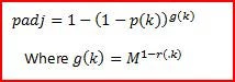
As an example, suppose we test for the impact of a program on five different outcomes, and obtain unadjusted p-values of 0.03, 0.05, 0.08, 0.24 and 0.50. Let’s consider the adjusted p-value for the first outcome (whose unadjusted p-value is 0.03). If the 5 outcomes are independent, then r(.1)=0, and then the procedure reverts to the Bonferroni adjustment: the adjusted p-value will be 1-(1-0.03)^5 = 0.14. If the 5 outcomes are all perfectly correlated, the adjusted p-value is equivalent to the unadjusted p-value of 0.03. And if the average correlation among the other outcomes is 0.5, the adjusted p-value will be 1-(1-0.03)^2.23 = 0.066.
I like how easy to use this procedure is, although the downside is that it is an ad hoc fix, that is only an approximate fix. It seems to perform reasonably well in simulations when the correlation among outcomes is fairly low (
Postscript: Jenny let me know you can also calculate these online at the Simple Interactive Statistical Analysis (SISA) website with discussion here.

Join the Conversation