All this confinement is triggering a lot of existential meditations for everyone. A friend recently asked about randomization inference in difference-in-differences with staggered rollout. This is a legitimate source of confusion—so it was time for a Development Impact blog post (and a new Shiny dashboard!) about this.
Event study designs and randomization inference
To answer this we first needed to question everything. It’s now common to see event studies where different units receive treatment at different times (and some not at all), with dynamic effects and (of course) flat pre-trends. What’s random in these analyses? And which variation in the data generates the estimates?
In recent blogs we’d separately experimented with potential sources of bias in event study designs and with randomization inference to account for spatial correlation in cross-country regressions. In this one, we’ll tackle randomization inference in event study designs, and insights for the interpretation of event study estimates.
Dashboards as the econometric sandbox
To answer these questions, we set out to create a simple to use tool for us to experiment with different methods under different assumptions about the data generating process. We started by simulating data, to see which specifications work when and under what assumptions they break down (e.g., what types of selection bias our estimates?).

To share these simulations without requiring a bunch of supplementary steps to download and execute code… we created a dashboard! The dashboard does three things. First, it enables varying the parameters of the data generation process. Second, it runs three simple approaches to randomization inference in event studies: assuming treatment and treatment timing are random, assuming only treatment timing is random, and dropping never treated units. And third, it visualizes and compares the estimates and inference coming out of each of these approaches. We found this useful as an exploration tool to understand what assumptions underlie different approaches to randomization inference in an event study design and the role of a pure control.
Data generating process
A series of sliders shift key components of the data generating process. These include the fraction of individuals that receive treatment, the true effect of the intervention, and, crucially, patterns of selection into treatment. The former two interact with different approaches to estimation and inference in event studies in surprising ways. The latter is the characteristics of units that are targeted by the policy, which crucially affects bias — do these units have different outcome levels? do they have differential trends?
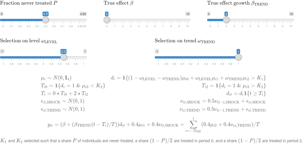
To simplify the analysis of randomization inference and the role of never treated units in estimation, we restrict to the case where there is 1) a set of control units that are never treated, and 2) a set of treated units, half of which are (randomly) targeted by the policy in period 0 and the other half of which are (randomly) targeted by the policy in period 2.
Models
We then run the following event study model on the data. Let \(y_{it}\) be the outcome of interest observed for unit \(i\) in period \(t\). Let \(\tau_{it}\) be the number of periods since \(i\) was treated (normalized to -1 for never treated units, and binned at -4 for all units more than 4 periods before treatment, and binned at 2 for all units more than 2 periods after treatment). We estimate
\[ y_{it} = \beta_{\tau_{it}} + \alpha_{i} + \theta_{t} + \epsilon_{it} \]
In contrast to our previous blog post, each of the event study estimates \(\beta_{\tau}\) can no longer be summarized as a single difference-in-difference estimator.
Sample selection To begin, we run this analysis on the full data, including never treated units, early treated units, and never treated units. Two sets of comparisons in this data enable estimation of event study coefficients. First, treated units are compared to never treated units; these comparisons are discussed in our previous blog post. However, never treated units may differ systematically from treated units, so these comparisons may introduce bias. Second, comparisons are made within treated units. The inclusion of this latter set of comparisons adds complication: for example, and as we discuss later, estimates may now be sensitive to how time periods are binned.
Next, we allow that never treated and treated units may not be on parallel trends, and drop never treated units from the analysis. Intuitively, estimates only depend on comparisons between treated units; we will use the dashboard to explore implications of this for bias.
Randomization inference To conduct potentially more robust inference, we apply randomization inference (discussed previously on this blog here, including links to discussions of some of its nice technical properties). Typically, this is used for experiments: when we know an intervention is randomly assigned, then we should estimate a zero-effect using random assignments that did not occur. Due to sampling noise, some estimates using these counterfactual random assignments will happen to be large; the share that are larger than our actual estimate gives us the p value associated with our estimate (we previously discussed randomization inference in non-experimental settings in this blog).
We begin by producing placebo estimates by randomly assigning both treatment and treatment timing across units (“Randomize Treated and Time Treated”). Implicitly, we assume that which units are never treated, early treated, and late treated was random. In addition, note that as all analysis includes individual fixed effects, we can think of this as assuming random assignment with respect to counterfactual trends (the familiar “parallel trends” assumption). This still allows never treated, early treated, and late treated units to have different levels of their outcomes (although this may suggest the parallel trends assumption is less credible).
Next, we produce placebo estimates by randomly assigning only treatment timing across units (“Randomize Time Treated”). Now, we assume that which units are early treated and late treated is random, but we allow that never treated units may be systematically different. If our estimates are driven by comparisons between treated and never treated units, then these placebo estimates may not be centered at 0, and therefore our estimator may yield a significant estimate even if the treatment had no effect.
Visualization, one click away!
Lastly, we plot the estimates from each of these approaches in the dashboard. All one needs to do is to click “Simulate!” to create a new simulation of data, run the event study and randomization inference, and plot the estimated coefficients, standard errors, and distribution of placebo coefficients from randomization inference under each approach. Voilà!

Now let’s play… threats to identification and inference!
Going back to our original motivation, how can we use randomization inference in event studies? This requires saying something about what is and is not random, and how these different sources of variation affect event study estimates. To experiment with this, we used the dashboard to simulate data after setting the true effect of the policy in the initial period and in pre-periods to 0 — this way, if we observe effects when the policy has no effect, we know the effects we estimate are actually caused by some source of bias. In addition, differences between randomization inference with both treatment and treatment timing randomized and randomization inference with only treatment timing randomized are informative about how these two sources of variation affect event study estimates.
We simulated four cases, two of which are visualized in the figure above. in our base scenario, we assume no effect of treatment (\(\beta = \beta_{\text{TREND}} = 0\)), no selection into treatment (\(\omega_{\text{LEVEL}} = \omega_{\text{TREND}} = 0\)), and that half of units are never treated (\(P = 0.5\)).
Selection on levels (\(\omega_{\text{LEVEL}} = 1\)): Third, any selection on levels does not generate bias.
Selection on trends (\(\omega_{\text{TREND}} = 1\)): Finally, selection into treatment on trends confounds our event study when we include never treated individuals, as these individuals are on different counterfactual trends. In this case, restricting to treated individuals removes this source of bias, under the assumption that treatment timing (conditional on ever being treated) is random with respect to counterfactual trends.
Fraction of units treated (\(\beta = 1\)): First, in the base case, both treatment assignment and treatment timing are random, and our model is correctly specified, so both models recover unbiased estimates. However, randomization inference randomizing only time treated when we include never treated observations does something weird: the placebo estimates are no longer centered at 0. Intuitively, this is because never treated units are included, and some interesting patterns emerge as one varies the fraction of units never treated (\(P\)).
Two notes on this. First, this is because the event study estimates are weighted averages of comparisons between treated units treated at different times, and between treated units and never treated units. Two recent papers (Goodman-Bacon, 2019; Sun & Abraham, 2020) formalize this decomposition. Therefore, placebo estimates randomizing only treatment timing are not centered at 0 because of differences on average between treated and never treated units. Second, when comparisons between treated units and never treated units are included, it is no longer sufficient to assume treatment timing is as good as random: we need parallel trends assumptions to hold across treated and never treated units. This highlights that randomization inference can also be used as a placebo check: if we thought parallel trends only held among treated units, randomizing timing across treated units should yield a distribution of estimates centered at 0 if our estimator only depended on comparisons between treated units.
Lastly, it is worth noting that robust standard errors clustered at the unit level and randomization inference yield fairly similar p values. As we discussed on a previous blog, randomization inference will only yield correct p values if your assumptions about which variation is random are correct as well.
Trends in treatment effects (\(\beta_{\text{TREND}} = 2\)): While the above two examples may suggest it’s always a good idea to drop never treated units, this need not be the case. When the treatment effect grows linearly in time since treatment, binning time periods can introduce bias. This is because binning implicitly assumes treatment effects are constant past a certain period. Although this binning does not particularly affect estimates when never treated units are included, it dramatically affects estimates when never treated units are dropped, leading to the estimation of large spurious pre-trends. A recent paper highlights that this is because when all units are eventually treated, more than one reference period is needed to estimate the model. As we used just one reference period, this implies we could only estimate the model because of binning periods beyond 2 and before -4.
Main takeaways
Simulating data can be helpful to understand what assumptions the approaches you take are or are not valid. As shown in the example, including never treated can either cause or remove bias. As is now common practice (here’s one recent example), implementing both approaches and, crucially, plotting raw means is therefore valuable for demonstrating robustness.
Note: All codes from our Econometric Sandboxes blogposts are hosted here!


Join the Conversation