
Motivation
In a previous post we outlined methods to estimating bunching-free counterfactuals when individuals bunch below some costly policy threshold. Today, we discuss the economic meaning that can be recovered from these estimates. In particular, the distance individuals travel to bunch at a threshold tells us about their responsiveness to the change in incentives at the threshold.
This responsiveness of individuals to changes in incentives at the threshold captures a local price elasticity — that is, how much individuals near the threshold shift their choices in response to a change in prices. In economics, price elasticities of supply and demand are central objects of interest, as they tell us how prices and quantities in equilibrium are affected by shocks or policies. In this post (as in many applications of bunching), we’ll consider the use of bunching estimators to recover a labor supply elasticity — how workers change their choice of hours (quantity) in response to changes in their hourly wage (price).
Economics of nonlinear budget sets
To fix ideas, we can start with a simple example of a worker choosing how many hours to work, given the earnings schedule they face. We graphically represent the set of possible choices the individual may make (their “budget set”) in the graph below. The individual may choose any points in the feasible region (earnings below their schedule given their wages), but may not choose any points in the infeasible region (earnings above their schedule given their wages). As we’ve drawn this budget set, it’s somewhat different from the typical budget set in that it is nonlinear — it is kinked!, and above the kink the earnings schedule becomes flatter. This means the individual earns a high wage at low earnings (their earnings are increasing quickly in their hours worked), but a lower wage at higher earnings (their earnings are increasing slowly in their hours worked). This kink may appear when the marginal tax rate, and therefore net of tax wages, suddenly drop above an earnings threshold.

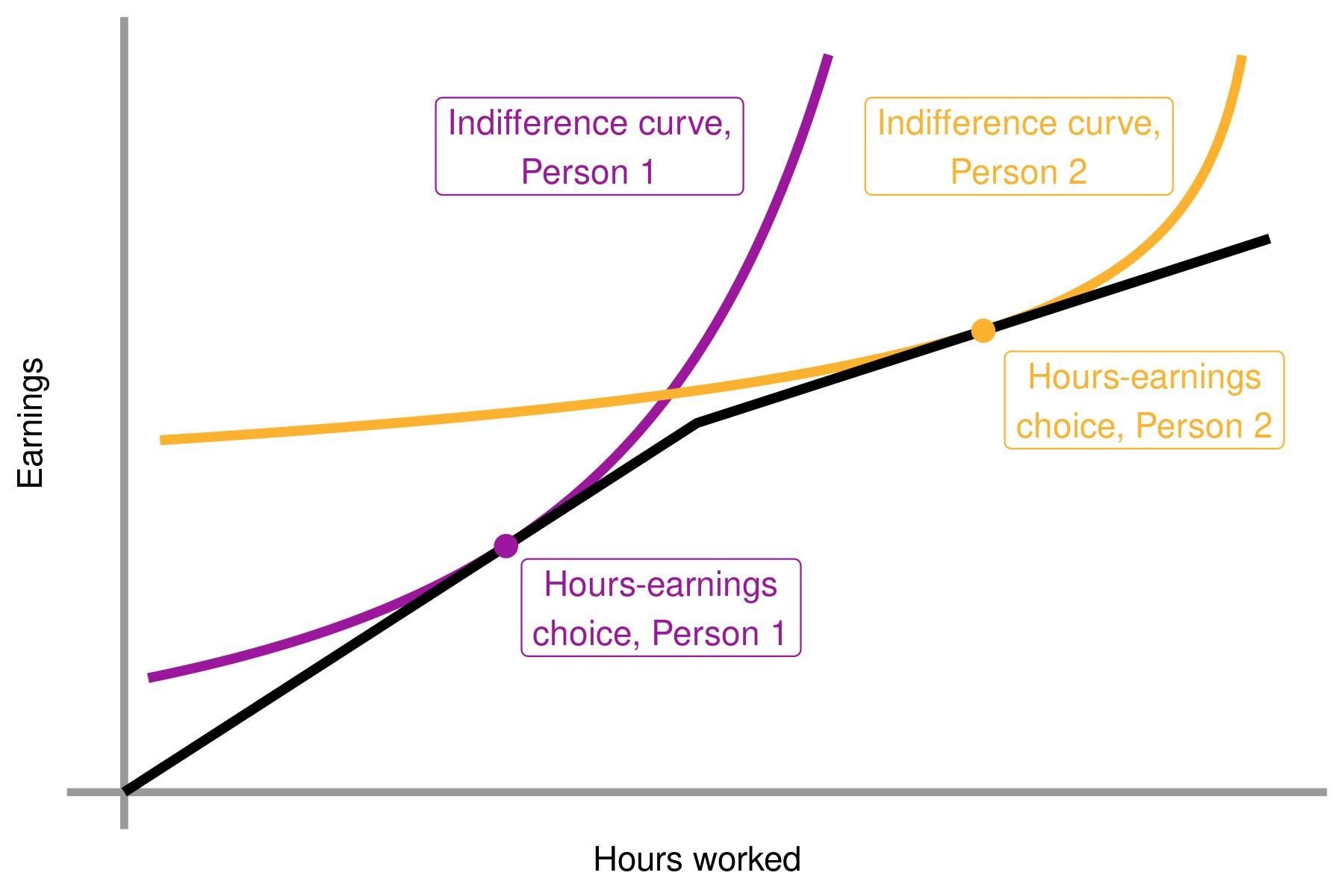
Individuals facing this budget set, on their set of possible choices of earnings and hours worked, must then choose the number of hours they will work (and in turn their earnings). These choices will depend on individual preferences and/or abilities—two individuals facing this same budget set may choose different hours, as individuals who place a strong value on earnings (relative to leisure) will tend to choose larger numbers of hours worked all else equal. We can represent these differences in individual preferences using indifference curves — the sets of points that a given individual places equal value on. Recall that each individual would then prefer to be on their highest possible indifference curve as, all else equal, individuals would prefer to have more earnings. Individuals then select a point where their indifference curve is tangent to the budget set, as tangency implies there is no feasible higher indifference curve. In the figure below, we provide an example of two individuals making different choices facing the same budget set — Person 1 locates below the kink, choosing fewer hours and lower earnings, while Person 2 locates above the kink, choosing more hours and higher earnings (no, we do not need to judge).
In the example above, we can see that different preferences lead to different choices. Similarly, different budget sets would lead to different choices: for example, individuals may increase their hours worked in a response to an increase in wages. How individuals will respond to a change to the budget constraint will depend crucially on the shape of their indifference curve. For example, individuals with very flat indifference curves can easily substitute hours and earnings, as the rate at which they are willing to trade hours for earnings is very stable. This then implies that a small change in wages can cause a large change in hours.
Recovering elasticities from bunching at a kink
How does this all relate to kinks? Formally, a kink is a sudden change (almost always decrease) in the slope of the budget set. In our example, this corresponds to a decrease in wages above an earnings threshold. As mentioned above, this decrease in wages will cause individuals who would have earned above the threshold without the kink to decrease their hours worked. However, this decrease in wages will have no effect on individuals who would have earned below the threshold. This discontinuous effect on individuals incentives, and in turn behavior, is what allows us to recover how responsive individuals are to wage changes.
Importantly, kinks will (in theory) cause some individuals above the threshold to shift exactly to the threshold, but never below the threshold, and it is this property that generates bunching! To see this graphically, we consider the thought experiment illustrated in the figure below — suppose we have initially a linear tax schedule (no kink) and then imagine that the government introduces a higher marginal tax above the threshold, decreasing wages past the threshold. This implies that the budget set changes from the solid line to the dotted line above the threshold. We have plotted two sets of indifference curves on the graph, in pink and orange. While the orange individual chooses higher hours and higher earnings with the linear budget set, both the orange and the pink individual choose to locate exactly at the kink with the kinked budget set. With many individuals, this manifests in the density graph below — individuals who would have earned above the kink shift their earnings to locate exactly at the kink.
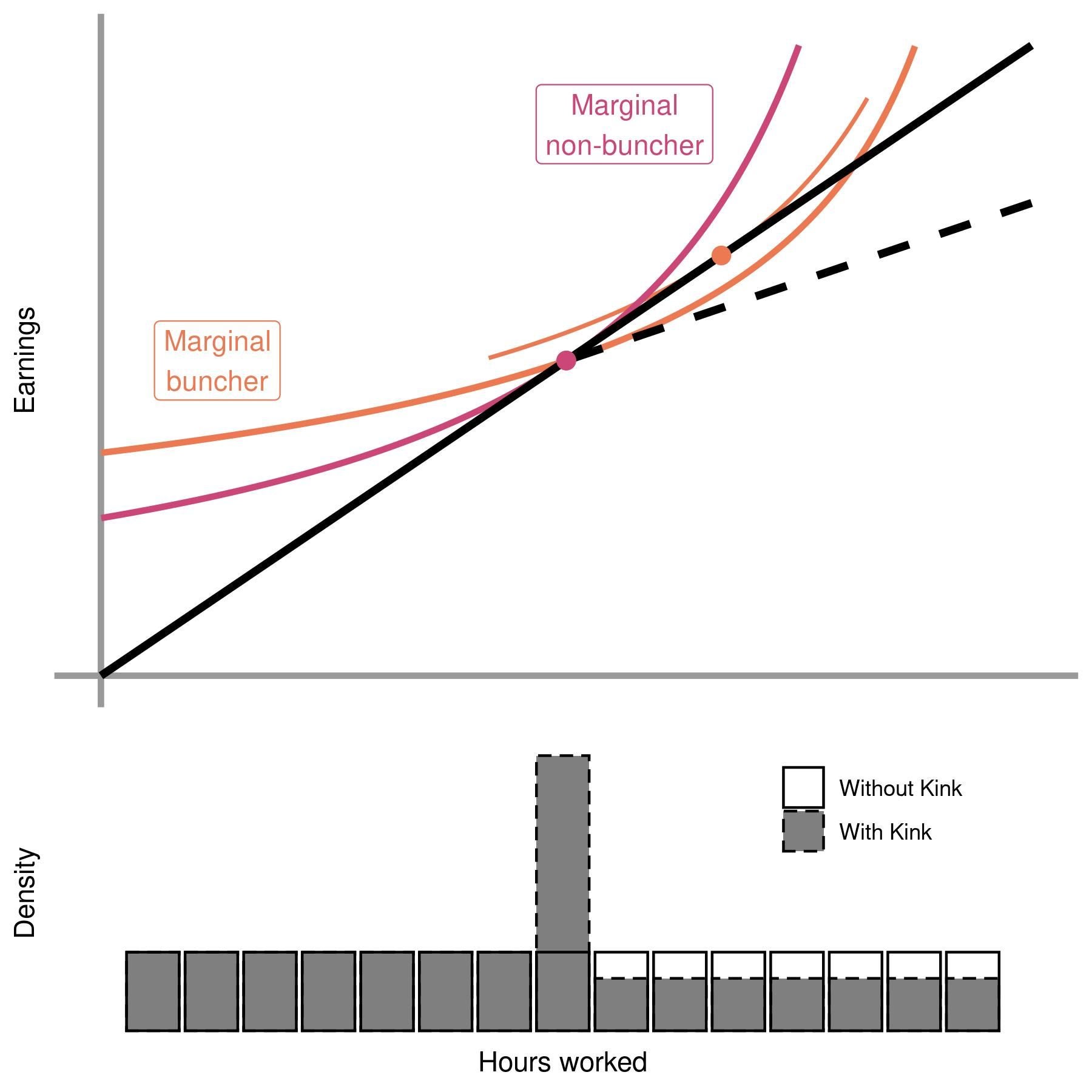
Next, the number of individuals who locate at the kink is informative about how responsive individual earnings are to (net-of-tax) wages. Intuitively, if individuals are more responsive, the decrease in wages above the kink will cause larger decreases in individuals’ hours worked, and cause more individuals to shift to the kink. To calculate an exact elasticity, the individuals depicted in orange and pink now play special roles. If the marginal tax rate was any lower above the threshold (i.e., if the wage was any higher above the threshold), the “Marginal buncher” would choose to be above the kink. In that sense, the “Marginal buncher” is the “last” individual to locate at the kink. In contrast, the “Marginal non-buncher” is the “first” individual to locate at the kink. Therefore, the excess mass at the kink is exactly the mass of individuals in between the “Marginal buncher” and the “Marginal non-buncher”!
The final step relates back to the econometrics discussed in the last blog — if we knew what the density of individuals would be without the kink, we would know how far the marginal buncher shifted their hours to reach the kink, which (as described previously) would tell us the labor supply elasticity of the marginal buncher. Recall that estimating this counterfactual density is exactly what bunching estimators do!
There are a number of challenges to the interpretation of elasticities from bunching at a kink. First, the approach described implicitly assumes all individuals have the same elasticity; otherwise, two individuals with the same earnings when the budget set was linear might make different choices about whether or not to bunch. Luckily, it turns out that even with heterogeneity, we still recover a particular average elasticity (Kleven, 2016). Second, all this assumes that economic agents are fully informed and can perfectly adjust their hours worked, leaving no room for optimization frictions. In practice individuals might not be aware of where the threshold is located or unable in the short-term to adjust their hours worked (due to fixed costs such as set number of hours worked, or changing jobs). As evidence of this, Chetty et al. (2011) show that kinks leading to a larger changes in marginal prices also produce higher estimates of elasticity parameters as individuals have larger incentives to incur these fixed adjustment costs. In another paper, Chetty et al. (2013) also directly shows that the amount of bunching at the kink of the EITC (the largest US transfer program) is an accurate measure of taxpayers’ knowledge about the tax code at the level of a neighborhood.
Recovering elasticities from bunching at a notch
As an alternative, a second form of sudden change in budget sets that causes bunching is a notch. While a kink is a sudden change in the slope of a budget set, a notch is a sudden change in the level of a budget set. We graphically represent an example of a notch in the graph below — in this case, once the individual’s earnings rise above a certain threshold, the individual experiences a sudden decrease in earnings! Think of this as a lump sum fee that one only needs to pay above a certain threshold, or a discrete benefit that suddenly disappears above a certain threshold. This actually creates a region above the threshold where no individual should want to be, as their hours worked would be higher but their earnings would be lower. This is an important feature of notches that we’ll return to shortly.
Similar to kinks, notches will (in theory) cause some individuals above the threshold to shift exactly to the threshold, but never below the threshold, and it is this property that generates bunching! To see this graphically, we illustrate the following thought experiment in the figure below — suppose we initially have a linear tax schedule (no notch) and then imagine that the government introduces a lump sum tax above the threshold, decreasing earnings past the threshold (but keeping wages the same). This implies that the budget set changes from the solid line to the dotted line above the threshold. We have plotted two sets of indifference curves on the graph, in pink and orange. While the orange individual chooses higher hours and higher earnings with the linear budget set, both the orange and the pink individual choose to locate exactly at the notch with the notched budget set. With many individuals, this manifests in the density graph below — individuals who would have earned above the notch shift their earnings to locate exactly at the notch! Just as for kinks, we can use the change in hours of the “Marginal buncher” (in orange) to recover the labor supply elasticity of the marginal buncher, and we can recover this change under the assumptions discussed in the previous post.
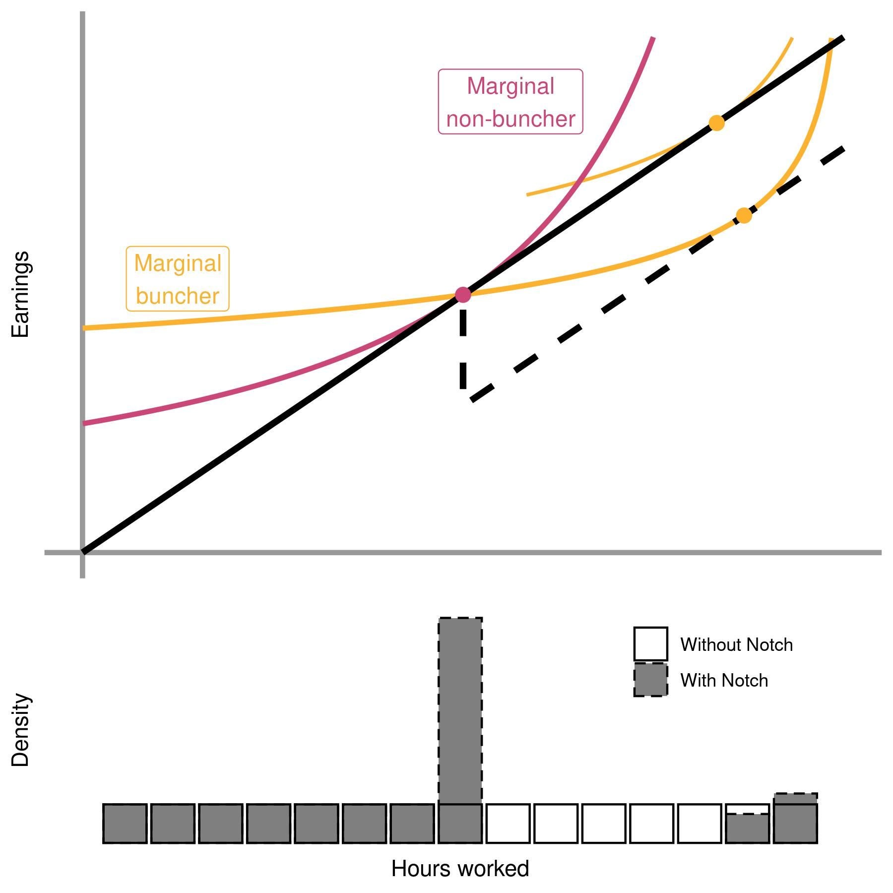
A crucial difference from a kink is that a notch produces a “dominated region”, where individuals have lower earnings despite working higher hours. In the figure above, this dominated region manifests as missing mass above the notch, where no individuals should choose to locate. As noted by Kleven & Waseem (2013), in practice the “dominated region” provides us with extra information — if we observed individuals who still report earnings in this “dominated region”, we would know these individuals must not be responsive to changes in the budget set, either because they are uninformed or because they face large adjustment costs! This extra information can be sufficient to recover how individuals would have responded with no adjustment frictions, which in turn allows us to recover individuals’ “frictionless elasticity”. Together, these estimates of adjustment frictions and the frictionless elasticity are necessary to know how individuals would respond to alternative changes to the budget set, which may be much larger (so frictions become less important) or much smaller (so frictions become more important) than the change at the notch.
Additional practical notes
- Estimation extensions In practice, when estimating the number of individuals who bunch, additional restrictions implied by the model can improve estimation. For example, a restriction for notches that excess mass below the notch is equal to missing mass above the notch can allow data driven selection of the window of manipulation. Best practices for the exact estimation approach is an empirical question, that depends both on the context, the budget set (kinked or notch), and any additional information that can help estimation (e.g., a pre-period before the introduction of the kink or notch, variation in how informed individuals are about the kink or notch); Kleven (2016) provides a recent review of these methods.
- Unknown price change In some settings, the change in incentives at a kink or a notch is instead unknown. For example, above an earnings threshold, individuals may lose access to a benefit of unknown value to those individuals. In that case, as an alternative, analogous to how a known change in incentives makes it possible to recover an unknown elasticity, a known elasticity would allow us to recover the unknown change in incentives.


Join the Conversation