Berk raised an existential question a few weeks back — should we consider deviating from the canonical 50% treatment/50% control RCT design when we expect treatment affects the variance, and not just the level, of outcomes? In theory, the 50/50 design can leave crucial statistical power on the table in this case, as there are efficiency gains from assigning additional observations to the study arm with higher variance in order to improve the precision with which its average outcome is estimated.
In this blog, we assess the size of the inefficiency caused by this potential misallocation of experimental treatment units. TL;DR: overall, our take is that power gains are unlikely to be large enough to justify deviating from the balanced 50/50 design — of course, there may be exceptional cases (we provide some examples later in the blog)! First, the 50/50 design is the most robust, in the sense that across all possible variances of outcomes in treatment and control, it minimizes the percentage increase in minimum detectable effects (MDE) relative to the optimal design. Second, in the binary case, power for the null of no effect is mechanically highest when average outcomes under treatment and control are the most different, but this is also the case when the variances are the most different. Hence, power is unlikely to be a concern in many cases where the optimal design is meaningfully different from 50/50. Third, in the continuous case, we provide guidance for when treatment is likely to affect variance — in particular, we show that when quantile treatment effects are increasing (decreasing), then treatment increases (decreases) variance. Fourth, we investigate this empirically in the context of microfinance RCTs, as microfinance is known to have increasing quantile treatment effects on profits (Meager, 2020). Even in this case, across 7 experiments the 50/50 design increases MDE by at most 18% relative to the optimal design.
How much can this possibly matter in theory?
Throughout this blog post, we’ll consider the example of the design of a microfinance RCT, where individuals \(i\) are randomly assigned to receive access (Treatment, so \(D_{i} = 1\)) or no access (Control, so \(D_{i} = 0\)) to microfinance loans, and to simplify we’ll assume there are no spillovers. We’ll focus on estimating the average impact of microfinance on individual business profits, \(\mathbf{E}[Y_{i}(1) - Y_{i}(0)]\), where \(Y_{i}(d)\) denotes individual \(i\)'s potential outcome if they receive treatment assignment \(d\) (so \(Y_{i}(1)\) is profits if you receive a microfinance loan, and \(Y_{i}(0)\) is profits if you don’t). As is standard, we can only observe \(Y_{i}(D_{i})\), individual \(i\)'s profits under their realized treatment assignment.
To estimate this average impact as precisely as possible, we are choosing to assign \(N_{0}\) individuals to control and \(N_{1}\) individuals to treatment. Under this assignment, the variance of our estimate of the average impact can be written as
\[\text{Var}[\overline{Y}_{1} - \overline{Y}_{0}] = \frac{\text{Var}[Y_{i}(0)]}{N_{0}} + \frac{\text{Var}[Y_{i}(1)]}{N_{1}}\]
where \(\overline{Y}_{d}\) denotes the sample mean of individuals assigned to treatment status \(d\). This generalizes the usual power formulas to allow the variance of outcomes under control and treatment to differ, as Berk discussed a few weeks ago.
To maximize our precision, we choose the fraction to assign to treatment holding fixed the total number of observations. Solving for this optimal fraction yields
\[\frac{N_{1}^{*}}{N_{0}^{*} + N_{1}^{*}} = \frac{\text{SD}[Y_{i}(1)]}{\text{SD}[Y_{i}(0)] + \text{SD}[Y_{i}(1)]}\]
In other words, the optimal number of individuals to assign to treatment is proportional to the relative standard deviation of outcomes under treatment. So, if treatment increases the variance of outcomes, we could improve precision by assigning more individuals to treatment.
Returning to our question now—how much can this possibly matter in theory? We can do a worst case analysis, calculating the maximum possible ratio of the standard error under a given design to the standard error under the optimal design, as a measure of the robustness of the given design. In other words, this asks: “in the worst case scenario, by what percent could I have decreased my minimum detectable effect by using the optimal design, instead of the selected design?”. For example, when we assign 50% of observations to treatment, in the worst case (as either the relative variance under control or the relative variance under treatment approaches 0), this ratio is 41%. It turns out this is the most robust of any design — this ratio is larger for any design other than 50% treatment/50% control. Considering this robustness is important — although we focus on a single outcome (profits) in this post, in practice most RCTs have multiple outcomes of interest, and treatment may increase and decrease the standard deviation for different outcomes.
If this matters with a binary outcome, you probably have sufficient power and need not bother!
When outcomes are binary, the standard deviation of outcomes is a straightforward function of the mean outcome. As a result, when anticipated treatment effects on a binary outcome are small, the impact of treatment on the standard deviation of outcomes will also be small, and the optimal design will be close to 50% treatment/50% control. In contrast, when anticipated treatment effects are large, the optimal design may deviate from 50% treatment/50% control, but power is likely to be high in these cases. As a result power gains for the null hypothesis of no treatment effect will typically be small once the sample is sufficiently large.
To provide an example, suppose the average outcome is .050 in the control group, and treatment increases outcomes; this generates relatively large potential power gains from the optimal design, as potential power gains are largest when outcomes in either control or treatment are very close to 0 or 1. Despite this, with 100 observations, power gains from the optimal design are largest when treatment increases outcomes from 0.050 to 0.225, at just 3.9pp (from 74.8% to 78.6%). Alternatively, with 400 observations, power gains from the optimal design are largest when treatment increases outcomes from 0.050 to 0.128 at just 1.7pp (from 79.0% to 80.7%).
However, deviating from 50% treatment/50% control may be justified for alternative null hypotheses; this is most likely to be the case when the precise point estimate, rather than the sign, of effects on a single binary variable are of primary interest. This could be the case for a medical trial, for example, where the medicine being trialed needs to substantially outperform the placebo (e.g., a vaccine effectiveness trial, or a trial for a very expensive treatment). Alternatively, if we’re comparing cost effectiveness at increasing a binary outcome across treatment arms of different costs (see past discussions of this design here and here), the null is of a proportionately larger impact of the higher cost arm; power gains with large numbers of observations may also be possible in this case.
This could matter with a continuous outcome, when quantile treatment effects are strongly heterogeneous …
With a continuous outcome, treatment can independently shift average outcomes and the standard deviation of outcomes. As a result, for the null hypothesis of no effect, power gains from the optimal design may be large regardless of sample size. To understand when treatment might increase the standard deviation of outcomes, we note that we can think about increasing the standard deviation of outcomes as treatment stretching the distribution of outcomes — when treatment has large effects at high outcomes, and small effects at low outcomes, this will cause treatment to increase the standard deviation of outcomes.
Formally, let \(F_{d}^{-1}(q)\) be the inverse cumulative distribution function of outcomes under treatment status \(d\) evaluated at quantile \(q\) — this is sometimes known as the quantile function, and returns the \((100*q)\)th percentile of the distribution of outcomes. Let \(\text{QTE}(q) \equiv F_{1}^{-1}(q) - F_{0}^{-1}(q)\) be the quantile treatment effect at quantile \(q\), that is the effect of treatment on the \(q\)th quantile of outcomes (e.g., \(QTE(0.5)\) is the effect of treatment on the median outcome). Let \(\tau \sim U(0,1)\) be a uniform random variable on the interval from 0 to 1. Then, with some calculus, we can write
\[ \text{Var}[Y_{i}(1)] - \text{Var}[Y_{i}(0)] = \text{Cov}[\text{QTE}(\tau), F_{0}^{-1}(\tau)] + \text{Cov}[\text{QTE}(\tau), F_{1}^{-1}(\tau)] \]
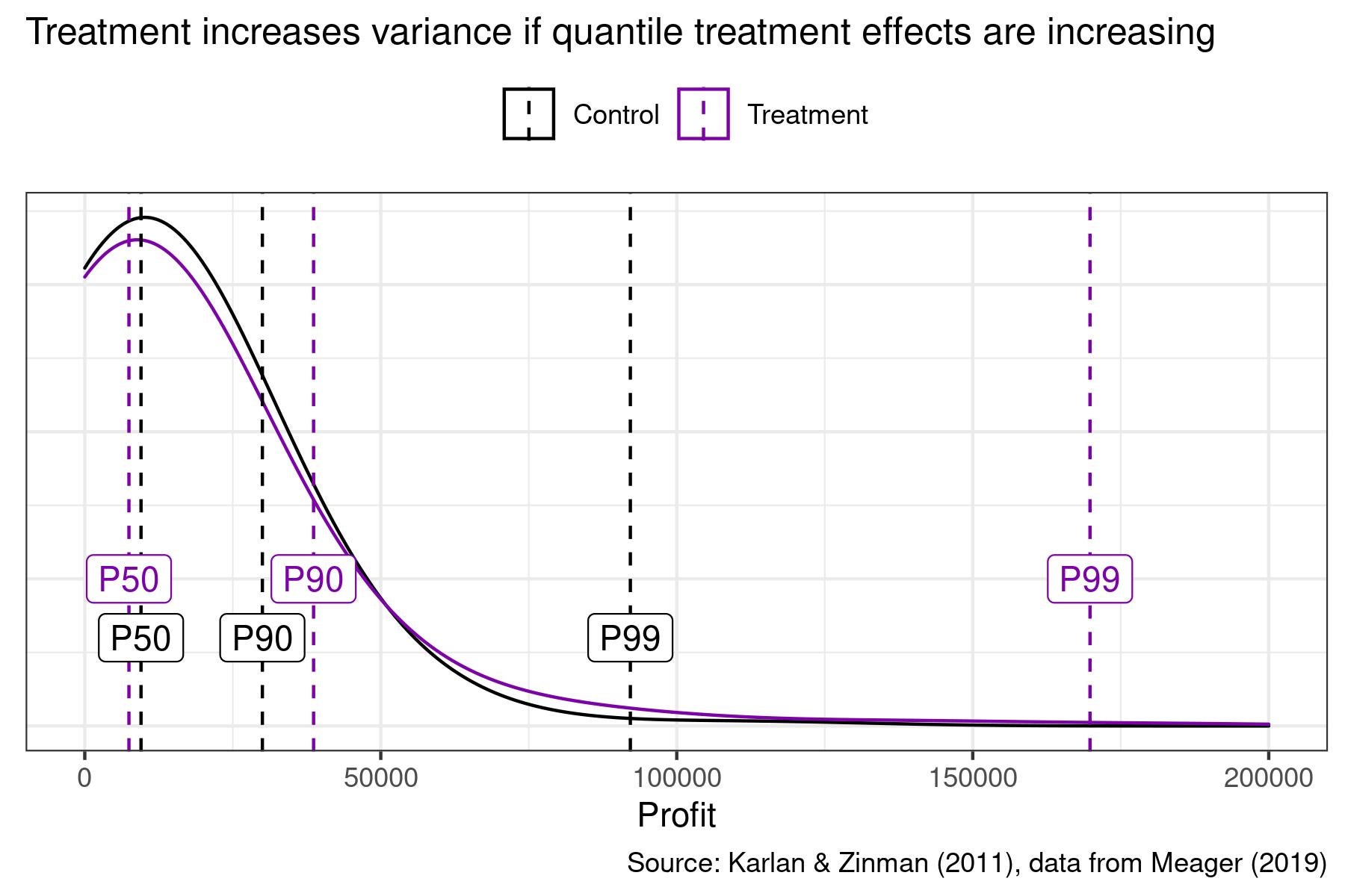
That is, the impact of treatment on the variance of outcomes is just a function of the covariance between quantile treatment effects and outcomes. Therefore, for example, when quantile treatment effects are increasing, treatment increases the variance of outcomes. We visualize this in the figure below using data from a microfinance RCT on business profits — quantile treatment effects are negative at the median, positive at the 90th percentile, and large at the 99th percentile. As a result, treatment increases the variance of business profits.
… yet, 50/50 does pretty well, even with an intervention where quantile treatment effects are strongly heterogeneous!
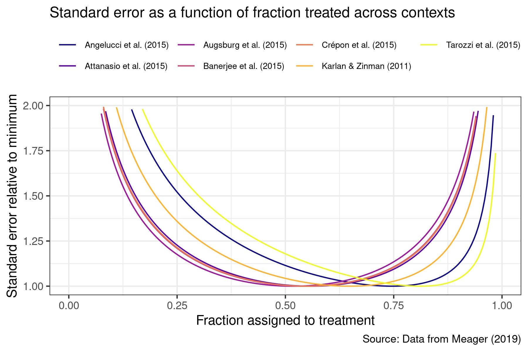
Empirically, how much is the impact of treatment on the variance of outcomes likely to matter with continuous outcomes? To answer this, we take advantage of strong evidence of systematically increasing quantile treatment effects of microfinance on business profits from Meager (2020) to see how much precision could be gained in microfinance RCTs for impacts on business profits by allocating more observations to treatment. Below, we plot the ratio of standard errors with different fractions assigned to treatment as a fraction of the standard error under the optimal design.
Across the 7 RCTs, the optimal fraction assigned to treatment ranges from 52% from Augsburg et al. (2015) to 81% from Tarozzi et al. (2015) — this highlights that it may be difficult to anticipate the optimal fraction to assign to treatment in any individual RCT. Despite this, assigning 50% to treatment and 50% to control increases standard errors by at most 18% (for Tarozzi et al. (2015)). As reference, assigning 67% to treatment and 33% to control performs best, increasing standard errors by at most 5%. Some power gains may therefore be possible from assigning more units to the arm with higher variance, but empirically these gains may be small even for an outcome where we have strong prior reason to anticipate treatment should impact the variance of outcomes.


Join the Conversation