A lot of us have been asking: “I have this event thing I am trying to estimate the impact of — so do I run an event study? Do I run a regression discontinuity in time? How about difference-in-differences? What are their respective identifying assumptions?” This is a legitimate source of confusion—so it was time for a Development Impact blog post (and a new Shiny dashboard!) about this.
Panel data
Fundamentally, these approaches all take advantage of changes in policy over time to estimate the impacts of a policy. In particular, we can compare outcomes for treated units (targeted by the policy) to outcomes for control units (not targeted by the policy), before and after the policy change. Past posts on this blog discuss constructing “synthetic controls” for treated units and running event studies and difference-in-differences when units become treated in different periods, and a recent paper discusses running regression discontinuity in time when comparisons are made just before and just after the implementation of the policy.
So what happens when we misspecify things and run the wrong model… For example, suppose we try to run a regression discontinuity in time when the impacts of the policy start small and grow progressively? Or we choose to estimate an event study when the policy specifically targets units that are on positive growth trajectories?
Dashboards as the econometric sandbox
To answer these questions, we set out to create a simple to use tool for us to experiment with different methods under different assumptions about the data generating process. We started by simulating data, to see which specifications work when and under what assumptions they break down (e.g., what types of selection bias our estimates?).

To share these simulations without requiring a bunch of supplementary steps to download and execute code… we created a dashboard! The dashboard does three things. First, it enables varying the parameters of the data generation process. Second, it runs the three main models we have in mind here: event study, regression discontinuity in time (RDiT), and difference-in-differences (DID). And third, it visualizes and compares the estimates coming out of each of these models. We found this useful as an exploration tool to understand what assumptions underlie different approaches to estimating policy impacts in panel data.
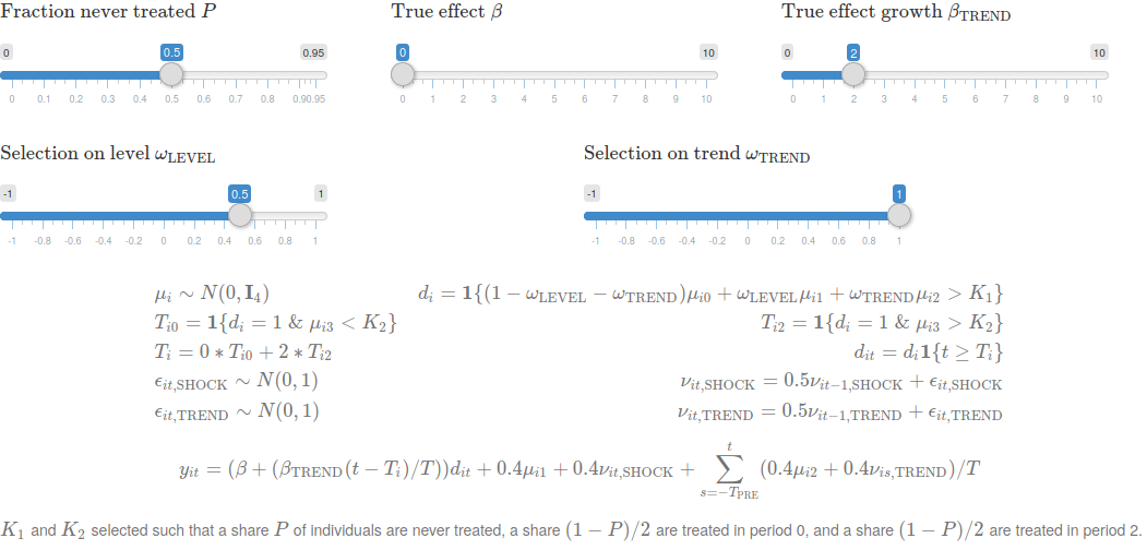
Data generating process
A series of sliders shift key components of the data generating process. These include the number of time periods and individuals, the true effects of the policy, properties of the structural errors, and, crucially, patterns of selection into treatment. The latter is the characteristics of units that are targeted by the policy, which crucially affects bias — do these units have different outcome levels? do they have differential trends? did they experience differential shocks, either to the level of their outcomes or to their trends, in the first period of the policy?
To focus on impacts of patterns of selection on each of the different estimators, we restrict to the case where there is 1) a set of control units that are never treated, and 2) a set of treated units that are all targeted by the policy in period 0.
Models
Next, we run three models on the simulated data. The first is a difference-in-differences (in purple). Letting \(y_{it}\) be the outcome of interest observed for unit \(i\) in period \(t\), and \(d_{it}\) be an indicator that the unit is treated and the policy has started, we estimate
\[y_{it} = \beta d_{it} + \alpha_{i} + \theta_{t} + \epsilon_{it}\]
This regresses the outcome on a treatment indicator, controlling for unit and period fixed effects, and our estimated \(\beta\) is the estimated effect of the policy. As discussed previously on this blog, difference-in-differences in this case estimates the change in outcomes for treated individuals minus the change in outcomes for control individuals, after relative to before the policy.
The second is an event study design (in black), the most flexible of the three approaches we consider, which allows both the impacts of the policy to change over time and also tests flexibly for differential selection into treatment in periods before the start of the policy. Here, letting \(\tau_{it}\) be, for unit \(i\) in period \(t\), the number of periods since unit \(i\) was treated (normalized to -1 for control units), we estimate
\[y_{it} = \beta_{\tau_{it}} + \alpha_{i} + \theta_{t} + \epsilon_{it}\]
In this case, each of the event study coefficients \(\beta_{\tau}\) is a simple difference-in-differences estimator, using the period just before the policy starts as the “before” period, and the period of the event study coefficient as the “after” period.
The third, regression discontinuity in time (in pink), is simply a differences-in-difference estimator which restricts to using a small number of periods before and after the policy starts. A recent paper discusses the choice of this number of periods and alternative functional forms for estimating policy impacts in regression discontinuity in time specifications.
Note that regression discontinuity in time and difference-in-differences coefficients are averages of event study coefficients; this is visualized in the dashboard by showing purple and pink lines (for difference-in-differences and regression discontinuity in time, respectively) over the range of event study coefficients that these average over.
Visualization, one click away!
Lastly, we plot the estimates from each of these models in the dashboard. All one needs to do is to click “Simulate!” to create a new simulation of data, run the three models, and plot the estimated coefficients and standard errors from each model. Voilà!

Now let’s play… threats to identification!
Going back to our original motivation, what patterns of selection cause bias in each of the three different approaches to estimation? To estimate the role of each, we used the dashboard to simulate data after setting the true effect of the policy to 0 — this way, if we observe effects when the policy has no effect, we know the effects we estimate are actually caused by selection bias.
We simulated four cases, visualized in the figure above.
Selection on level: First, when the policy targets units with higher levels of outcomes, all methods recover the true null effect — this is because the within individual differencing in each estimator eliminates bias caused by targeted individuals having higher outcomes than others.
Selection on trend: Second, when the policy targets units with higher growth in outcomes, estimates of the effect of the policy are positive and grow (when they should all be 0). However, from the event study coefficients, we can see a failure of the familiar “parallel trends” assumption — treated units and control units were on different growth paths even before the start of the policy.
Selection on shock: Third, when the policy targets units that experience a positive shock in the period the policy starts, all approaches yield biased estimates. This would be the case, for example, if we compared unemployed to employed individuals to evaluate a policy targeted at reducing unemployment on earnings, as unemployed individuals have likely recently received a negative shock to their earnings. In practice, applied researchers often use placebo checks to test for this concern — continuing with the unemployment example, higher frequency data would allow observing that the targeted (unemployed) individuals experienced a negative shock before the policy started, which would appear as a violation of parallel trends.
Selection on trend shock: Fourth is when the policy targets units that experience a positive shock to the growth in their outcome in the period the policy starts. In this case, the event study shows parallel trends before the start of the policy, but the estimated effects of the policy are biased and appear to grow over time. However, as selection is driven by shocks to growth in outcomes (and not shocks to levels of outcomes), regression discontinuity in time estimators are less biased that difference-in-difference estimators. In practice, this case may be very rare — it is quite difficult to anticipate which units are likely to have disproportionately high growth in practice and to target based on this. Additionally, applied researchers are often able to allow for this possibility by including time trends to flexibly differ across units with different observable characteristics.
Main takeaways
Estimating more flexible models (e.g., event study instead of regression discontinuity in time or difference-in-differences) as a first pass helps to understand the underlying structure of the data and permits quick checks of key identifying assumptions. Simulating data can be helpful to understand under what assumptions the approaches you take are or are not valid. For example, here we can see that when units select into treatment in response to shocks to their trend, standard parallel trends checks will pass, but estimates of long run impacts will be biased (although estimates of short run impacts will be less biased). The validity of these identifying assumptions will be fundamentally specific to the underlying context.
Note: All codes from our Econometric Sandboxes blogposts are hosted here!


Join the Conversation