
Results from the ICP are available at icp.worldbank.org. This blog series, edited by Edie Purdie, covers all aspects of the ICP and explores the use made of these data by researchers, policymakers, economists, data scientists, and others. We encourage users to share their data applications and findings in this blog series via icp@worldank.org.
As many readers know, the International Comparison Program (ICP) produces purchasing power parities (PPPs) and comparable price level indexes for each of its 170-plus participating economies, as well as PPP-based volumes and per capita measure of gross domestic product and its expenditure components. PPPs convert different currencies to a common currency and, in the process of conversion, equalize their purchasing power by controlling for differences in price levels between economies and provide a measure of what an economy’s local currency can buy in another economy.
There are many phases to the ICP’s PPP production process, including multistage calculations at the national, regional, and global levels. This blog is part of our ongoing outreach efforts focusing on transparency of the process and methods utilized in producing the program’s results. It is the second blog in the Demystifying ICP Purchasing Power Parity calculations using Python series. Together these blogs provide a fully transparent record of the calculation process
The first blog outlined the steps for estimating PPPs for countries within a single region, as calculated by the ICP Regional Implementing Agencies. This second blog focuses on the procedure for linking regional PPPs into a global set of PPPs. We use again mock average price and expenditure data and carry out the calculation using Python, a free, open-source programming language.
For a detailed overview of the methodological steps for the computation and aggregation of PPPs between regions, please refer to the methodology section of the ICP website and to Chapter 26 “Linking and Calculation of Global Results” of the ICP Operational Guidelines and Procedures for Measuring the Real Size of the World Economy.
Example of estimating PPPs using Python
What follows are code excerpts, using a Jupyter notebook, which are sequentially organized to understand how global ICP PPPs are estimated. Click each tab to see the Python code applied at each step. The full notebook with the entire code set in an executable online environment is available here (no installations are required, but it may take some time to load the first few times).
Input Data
We start by loading the input datasets necessary for the calculations. These include annual national average price data, expenditure data, and regional PPPs. A review of the price and expenditure data required to estimate PPPs is provided in the World Bank Data Blog How does the ICP measure price levels across the world?
## Load libraries
import pandas as pd
import numpy as np
import statsmodels.api as sm
#Load price data
data = "price_data.csv"prices =pd.read_csv(data)
#Load regional PPPs data
datappp = "ppp_reg.csv"ppp_reg =pd.read_csv(datappp)
Frequent users of ICP data will recall that the ICP Classification of Expenditures breaks down expenditure on final goods and services into different levels, and defines 155 basic headings as the lowest level at which participating economies can estimate explicit expenditures. Each basic heading consists of a group of similar well-defined goods or services and is the lowest level for which PPPs are calculated. As in our previous blog, we focus on three basic headings (“bh”) as examples for our computation: garments, rice, and pork.
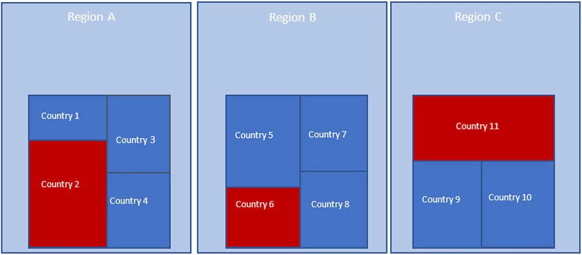
Furthermore, we use 11 countries in our example, each belonging to one of three different regions. Within the ICP framework, regions represent the first building block in the process of cross-country comparisons. The Regional Implementing Agencies are responsible for calculating regional PPPs based on the prices and national accounts expenditures provided by participating economies. Each region designates one country within their region as numeraire and regional PPPs are calculated in relation to this regional numeraire. In our example illustrated below, Country 2 is the numeraire for region A, Country 6 for region B and Country 11 for region C.
Global linking of regional basic heading PPPs
In order to estimate PPPs between regions we identify a global numeraire country. In the ICP, the United States of America acts as the global reference country. In our example, Country 11 acts as the global numeraire and region C as the reference region. It is worth noting how the choice of the base country does not influence the results, as the current PPP methodology ensures that estimates are base country-invariant, as explained below.
numeraire = 'C'
numeraire_c = 'country11'
Regional PPPs are then linked to the global numeraire via so-called “linking factors”. These are scalars estimated for each region via a regression method known as the “weighted region product dummy” (RPD-W).
The RPD-W method is carried out within each basic heading by regressing the logarithm of the observed country item prices, converted into a common regional numéraire using the country's regional basic heading PPPs, on item dummies (one for each item) and region dummies (one for each region other than the region of the global numeraire).
The RPD-W method also incorporates the country-reported item-level importance indicators with the idea of "down-weighting" less representative items during the calculation (for a detailed overview of how importance indicators are derived, see Chapter 20 of the Operational Guidelines and Procedures for Measuring the real size of the world economy report).
for bh in prices.bh.unique():
tempdf=prices[prices.bh == bh]
X=tempdf.loc[:, [x for x in tempdf.columns if x.startswith(('r_', 'i_'))]]
y=np.log(tempdf['price']/tempdf['ppp_reg'])
wts=tempdf['imp']
wts_cpd=sm.WLS(y, X,weights=wts)
res=wts_cpd.fit()
res_eparams=np.exp(res.params)
l_coef.append(res_eparams)
l_bh.append(bh)
coef = np.array(l_coef, dtype=float)
cols = list(X) #store column heads of X as a list
coef[coef == 1] = np.nan #%% replace PPPs that were exp(0)=1 with 'np.nan'
print("\n","Linking Factors:", "\n")
print(df_bhppp ,"\n")
| Linking factors: | ||||
bh |
region |
lf |
||
| garment | C | 1.000000 | ||
| pork | C | 1.000000 | ||
| rice | C | 1.000000 | ||
| garment | A | 8.003727 | ||
| pork | A | 26.377552 | ||
| rice | A | 81.814732 | ||
| garment | B | 1.543396 | ||
| pork | B | 11.786040 | ||
| rice | B | 17.856102 | ||
ppp_regLF=pd.merge(ppp_reg, df_bhppp, how=:'inner', on=( 'bh','region'))
ppp_regLF['ppp_linked']=ppp_regLF[ 'ppp_reg']*ppp_regLF['lf']
ppp_regLF = ppp_regLF.drop(['ppp_reg'], axis= 1)
ppp_regLF=ppp_regLF.pivot(index="bh",
ppp_regLF=ppp_regLF.pivot(index="bh",
columns="country",
values="ppp_linked").reset_index()
#Sort cols with numeraire as column1 and print
ppp_regLF=sorting(numeraire_c,ppp_regLF)ppp_reg =pd.read_csv(datappp)
print("\n","Global Basic Heading PPPs:", "\n")
print(ppp_regLF ,"\n")
| Basic Heading PPPs | ||||||
bh |
country11 |
country1 |
country10 |
country2 |
country3 |
country4 |
| garment | 1.0 | 77.984446 | 1.379874 | 8.003727 | 162.961045 | 0.757609 |
| pork | 1.0 | 365.986031 | 2.558659 | 26.377552 | 500.779254 | 2.420035 |
| rice | 1.0 | 1152.334562 | 2.822813 | 81.814732 | 859.978863 | 5.501386 |
bh |
country5 |
country6 |
country7 |
country8 |
country9 |
| garment | 1.888739 | 1.543396 | 7.262116 | 2.907029 | 95.197708 |
| pork | 4.597515 | 11.786040 | 24.609856 | 14.998082 | 97.780273 |
| rice | 5.896068 | 17.856102 | 76.714659 | 24.084759 | 422.305630 |
Above-basic heading aggregation
Once global linked basic heading PPPs are obtained by multiplying regional basic heading PPPs by linking factors, they are then aggregated using national accounts expenditure values in local currency units for each country as weights or volumes.
#Load basic heading expenditure values
#Should contain bh and countries with prefix c
code="bhdata_exp.csv"
df_bh=pd.read_csv(code,index_col="icp_bh")
The global aggregation method follows the same steps for the aggregation of PPPs at the regional level, as described in the previous blog. First, we construct bilateral PPPs for each pair of countries, using basic heading-level national accounts expenditure values as weights from each country in turn. A Laspeyres-type bilateral PPP is calculated between each pair of countries followed by a Paasche-type bilateral PPP. The geometric mean of the Laspeyres- and Paasche-type bilateral PPPs gives us the Fisher-type bilateral PPP between each pair of countries in the dataset.
##Calculate Laspeyres bilateral PPPs
shape = (len(df_bh.columns),len(df_bh.columns))
lp = np.zeros(shape)#square matrix: country x country
nrow=len(lp) # gets the number of rows
ncol=len(lp[0])
for row in range(nrow):
for col in range(ncol):
#weighted means by looping over df rows
lp[row][col]= np.average((ppp_regLF.iloc[:,row]/ppp_regLF.iloc[:,col]),weights= df_bh.iloc[:,col])
lp_ppp = lp
lp_ppp = pd.DataFrame(data = lp_ppp, index = df_bh.columns, columns =df_bh.columns
#Calculate Paasche bilateral PPPs
pa = np.transpose(np.reciprocal(lp))
pa_ppp = pd.DataFrame(data = pa, index = df_bh.columns, columns =df_bh.columns)
shape = (len(df_bh.columns),len(df_bh.columns))
fi = np.zeros(shape)#square matrix: country x country
nrow=len(fi) # gets the number of rows
ncol=len(fi[0])
for row in range(nrow):
for col in range(ncol):
fi[row][col]= nangmean([lp[row][col],pa[row][col]])
fi_ppp = pd.DataFrame(data = fi, index = df_bh.columns, columns =df_bh.columns)
Next, the Gini-Éltető-Köves-Szulc (GEKS) method is applied to the matrix of Fisher-type bilateral PPPs. GEKS PPPs are calculated between each country relative to the numeraire or base country. GEKS PPPs are considered “multilateral” because the GEKS procedure uses both direct and indirect PPPs and thus accounts for the relative prices between all the countries as a group.
#Calculate GEKS multilateral ppps
##requires the earlier nangmean function
geks = np.zeros(shape) # zero 'country x country' matrix
nrow=len(geks) # gets the number of rows
ncol=len(geks[0])
for row in range(nrow):
for col in range(ncol):
geks[row][col]= nangmean(fi[row]/fi[col])
geks_vec = np.zeros(shape=(1,len(df_bhexp.columns)))
# as we need a vec- tor of ppps, not a matrix
j=len(geks_vec[0])
for col in range(j):#..one PPP per country, or col of bhexp df
geks_vec[:,col]=nangmean(geks[col,0]/geks[0,0]) #ge-
omean over each row, w/ each col rebased to country in col1
geks_ppp = np.array(geks_vec)
geks_ppp = pd.DataFrame(geks_ppp)
geks_ppp.columns = df_bh.columns
#Reshaping the global GEKS data frame
geks_ppp = geks_ppp.melt(var_name="country",value_name="geks"
print("\n","GEKS Multilateral PPPs:", "\n")
print(geks_ppp ,"\n")
| GEKS Multilateral PPPs: | |||
country |
geks |
||
| country1 | 182.290597 | ||
| country2 | 14.604400 | ||
| country3 | 231.408276 | ||
| country4 | 1.222144 | ||
| country5 | 2.250524 | ||
| country6 | 3.023521 | ||
| country7 | 13.200933 | ||
| country8 | 5.624968 | ||
| country9 | 97.486266 | ||
| country10 | 1.631125 | ||
| country11 | 1.000000 | ||
The GEKS method is needed to make the Fisher-type bilateral PPPs transitive and base country-invariant. Transitivity means that the PPP between any two countries should be the same whether it is computed directly or indirectly through a third country. Base country-invariant means that the PPPs between any two countries should be the same regardless of the choice of base or numeraire country.
Country Aggregation with Redistribution procedure.
The final step in the process of global PPPs estimation consists of applying the Country Aggregation with Redistribution (CAR) procedure. This step is undertaken to guarantee the principle of fixity. Fixity implies that the relative volumes in the global comparisons between any pair of countries belonging to a given region should be identical to the relative volumes of the two countries established in the regional comparisons to which they belong.
In order to adhere to this principle, regional volume totals in the global comparison are obtained by summing the GEKS-adjusted volumes for individual countries in each region. These volume totals are then divided using the countries’ expenditure shares in regional comparison. Finally, PPPs in world numéraire for each country are derived indirectly by dividing countries' nominal expenditures by the volume-share adjusted expenditures.
#Merging the expenditure and global geks dataframe
car_df = pd.merge(volshare_df, geks_ppp, how = 'inner', on= ('country'))
#Converting the total exp using the global geks
car_df['inner'] =car_df['total_exp']/car_df['geks']
##Calculating the total regional expenditure in geks adjusted units
car_df['exp_gek_reg'] =car_df['exp_gek'].groupby(volshare_df['region']).transform('sum')
Applying the regional volume share to the total expenditure and re-basingit on the numeraire PPP
car_df['exp_adj']=car_df['exp_gek_reg']*car_df['volshare']
car_df['PPPglobal']=car_df['total_exp']/car_df['exp_adj']
car_df.set_index(car_df['country'], drop=True, append=False, inplace=True)
car_df['PPPglobal_num']=car_df['PPPglobal']/car_df.at['country11','PPPglobal']
print("\n","Global linked PPPs:", "\n")
print(car_df.PPPglobal_num ,"\n")
| Global linked PPPs: | |||
country |
PPPs |
||
| country1 | 183.235520 | ||
| country2 | 14.579824 | ||
| country3 | 239.182896 | ||
| country4 | 1.162493 | ||
| country5 | 2.214319 | ||
| country6 | 3.139569 | ||
| country7 | 13.982184 | ||
| country8 | 5.357493 | ||
| country9 | 101.858780 | ||
| country10 | 1.507351 | ||
| country11 | 1.000000 | ||
In the above example, we showcased the main steps to calculate global PPPs. Information about the overall ICP methodology is provided on the ICP website. Please do contact us at icp@worldbank.org for further discussion.

Join the Conversation