
Sometimes it might seem like millions of econometricians have been coming after difference-in-differences (see this summary of recent work), leaving us all wondering whether we can still run (let alone publish) difference-in-difference regressions? And if so, how?
In the end, as it often does, when difference-in-differences is (and isn’t) okay all hangs on one simple question — “What are we trying to estimate?” New work has clarified what difference-in-differences and related estimators estimate, and contrasts this with what they’re trying to estimate.
In this two-part blog, we try to demarcate old from new, and explain in simple terms what these new papers contribute to the estimation of difference-in-differences. We highlight that, in all cases discussed, the traditional difference-in-differences with pre- and post-, control and treatment, is left unscathed. In fact, this forms the fundamental building block of more complicated estimators that eliminate previously unknown bias in two way fixed effects implementations of difference-in-differences with many treated groups!
So, are our difference-in-differences designs fundamentally flawed? It depends!
When is TWFE okay? Canonical difference-in-differences
The traditional difference-in-differences design is two cohorts, two periods — one cohort is control in both periods, and the other cohort becomes treated in the second period. We plot one example of this below — in the example, Cohort 2 becomes treated after 2005 (and experiences a sharp increase in outcomes when it becomes treated), while Cohort 1 remains control in both periods.
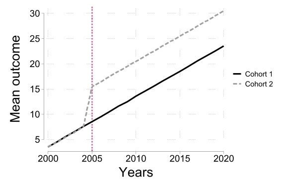
Identification of causal effects requires “parallel trends” — absent treatment, Cohort 1 and Cohort 2 would have had the same changes in outcomes (and usual SUTVA assumption). Under “parallel trends”, the change in outcomes in Cohort 1 (from pre-2005 to post-2005) is a valid counterfactual for what the change in outcomes in Cohort 2 (from pre-2005 to post-2005) would have been absent treatment (see past blogs on the parallel trends assumption here and here). Therefore, the difference-in-differences estimator of treatment effects is simply the difference between the change in outcomes in Group 2 and the change in outcomes in Group 1. Note that this approach generalizes naturally to cases where parallel trends only holds after we control for differences in characteristics across the two groups.
In this simple case, difference-in-difference estimators recover the average effect of treatment in the post period for Cohort 2, the “average treatment effect on the treated” or “ATT”. Two things to notice here. First, treatment effects may change over time (although in the example above, Cohort 2 experiences a constant ATT over time) — we do not know whether Cohort 2 would have the same ATT had we waited one more period before measuring post outcomes. Second, treatment effects may differ across groups — we do not know whether Cohort 1 would have had the same ATT as Cohort 2 in a given period.
It is common for researchers to implement the difference-in-difference estimator with two periods and two groups using two way fixed effects. Letting \(i\) index individuals and \(t\) index time periods, two way fixed effects estimates the impact of treatment D on outcome y by
\[ y_{it} = \beta^{\text{TWFE}} D_{it} + \theta_{i} + \delta_{t} + \epsilon_{it} \]
where \( \theta_{i} \) is an individual fixed effect, \( \delta_{t} \) is a time fixed effect, and \( \beta^{\text{TWFE}} \) is the two way fixed effects estimator of ATT. In contrast, letting \( C(i) \) denote the cohort of individual i, the difference-in-difference estimator of ATT (\( \beta^{\text{DID}} \)) can be implemented via the following regression
\[ y_{it} = \alpha + \beta^{\text{DID}} \mathbf{1} \{ C(i) = 2 \; \& \; t = \text{post} \} + \gamma \mathbf{1} \{ C(i) = 2 \} + \eta \mathbf{1} \{ t = \text{post} \} + \nu_{it} \]
It is well known that when there are two groups and two periods, \( \beta^{\text{TWFE}} = \beta^{\text{DID}} \) — that is, two way fixed effects and difference-in-differences recover identical estimates. As a result, two way fixed effects is valid under the same parallel trends assumption as difference-in-differences!
While it is straightforward to extend two way fixed effects to the case with multiple groups and multiple periods (we don’t even need to change the above specification!), generalizing difference-in-differences is less immediate. As a result, two way fixed effects is popular when there are multiple groups and multiple periods. This highlights two key ideas. First, that the traditional parallel trends assumption may also be challenging to generalize. Second, that there is clearly something restrictive about the two way fixed effects specification, as it implicitly imposes that ATT are identical across groups and across time periods by estimating a single \( \beta^{\text{TWFE}} \) !
So what exactly is TWFE doing when we have multiple cohorts and multiple time periods?
Tomorrow in Part 2, we will discuss recent work that describes the perils and pitfalls of this naive approach to extending difference-in-differences and proposes solutions. For today, we just go over the issue that's provoked such a wave of excitement in applied micro circles.
For this we extend our example above to the case of 3 cohorts, where two of them are now treated — Cohort 2 still in 2005, and also now Cohort 3 in 2010.

We now have 3 cohorts we can compare against each other, suggesting 3 possible comparisons — Cohort 2 against Cohort 1, Cohort 3 against Cohort 1, and Cohort 3 against Cohort 2. The first of these two comparisons correspond naturally to canonical difference-in-differences described above — Cohort 1 is control in both periods, and Cohorts 2 and 3 become treated in 2005 and 2010, respectively. The third comparison is more challenging — as both Cohort 3 and Cohort 2 become treated, this does not correspond to our canonical difference-in-differences setup. In tomorrow's blog we will show that the issue with TWFE stems from this comparison between treated cohorts …


Join the Conversation